Visualisation customs

Here we present researcher’s visualization customs and awareness about some methodological problems.

Setup

Code

data <- read_excel("../data/results_survey.xlsx") 

data <- data[1:121] %>% 
  filter(.[[18]] !='Yes') # not analysed any EEG method

font_add_google("Lato")
showtext_opts(dpi = 200)
showtext_auto(enable = TRUE)

Familiarity with plots

Recognition

Code

vec <- c("line", "butterfly", "topo",  "topo_map", "topo_array", "erp_image", "parallel", "channel_image")
familiar <-  data[61:68] %>% rename_at(vars(colnames(.)), ~ vec) %>% 
  mutate_at(vars(vec), function(., na.rm = FALSE) (x = ifelse(.=="Yes", 1, 0)))

rec <- data.frame(rowSums(t(familiar))) %>%  tibble::rownames_to_column(., "plot") %>% 
   rename_at(vars(colnames(.)), ~ c("plot", "sum_scores"))  %>% 
  arrange(., desc(sum_scores))

rec %>% 
  ggplot(data = ., aes(y = reorder(plot, sum_scores), x= sum_scores)) +
  geom_col(stat="identity", fill ="lightblue1", col="dodgerblue3") + ylab("plot") + theme_classic() + 
  geom_text(aes(label = sum_scores, group = plot), position = position_dodge(width = .9), hjust = -0.1) +
  theme(legend.position="none", plot.title = element_text(hjust = 0.5)) +
  labs(y = "Plot types", x = "Scores") + 
  ggtitle("Select plots you are familiar with") +
  labs(caption = sprintf("N of respondents - %d",  nrow(familiar))) +
  theme(legend.position="none", plot.caption.position = "plot", plot.caption = element_text(hjust=0), axis.text = element_text(size = 10))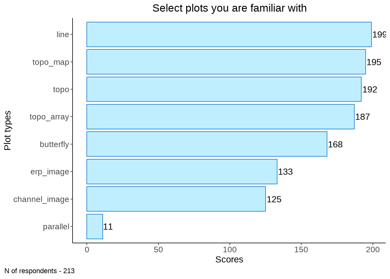

Code

familiar1 <- familiar %>%  mutate(n = rowSums(across(where(is.numeric))))
table(familiar1$n)  %>%  t() %>% data.frame()  %>% 
  mutate(percent_score = round(Freq / 213 * 100)) %>% 
  ggplot(., aes(y = Var2, x = percent_score)) +
  geom_col(stat="identity", fill ="#6BAED6") +
    labs(x = "", y = "Number of recognised plots", title = "Number of plots recognised by EEG researchers") + theme_classic() +
    geom_text(aes(label = paste0(percent_score, "%")), 
              position = position_dodge(width = .9), hjust = -0.2, size = 4) + theme(
      axis.text.y = element_text(size = 14),
      legend.position="none", plot.caption.position = "plot", 
      plot.caption = element_text(hjust=0), 
      text = element_text(family = "Lato"),
      axis.text.x = element_blank(), axis.text = element_text(size = 10),  
      plot.title = element_text(color = "grey10", size = 16, face = "bold"),
      axis.title.y = element_blank(),
      plot.title.position = "plot"
      ) + xlim(0, 45)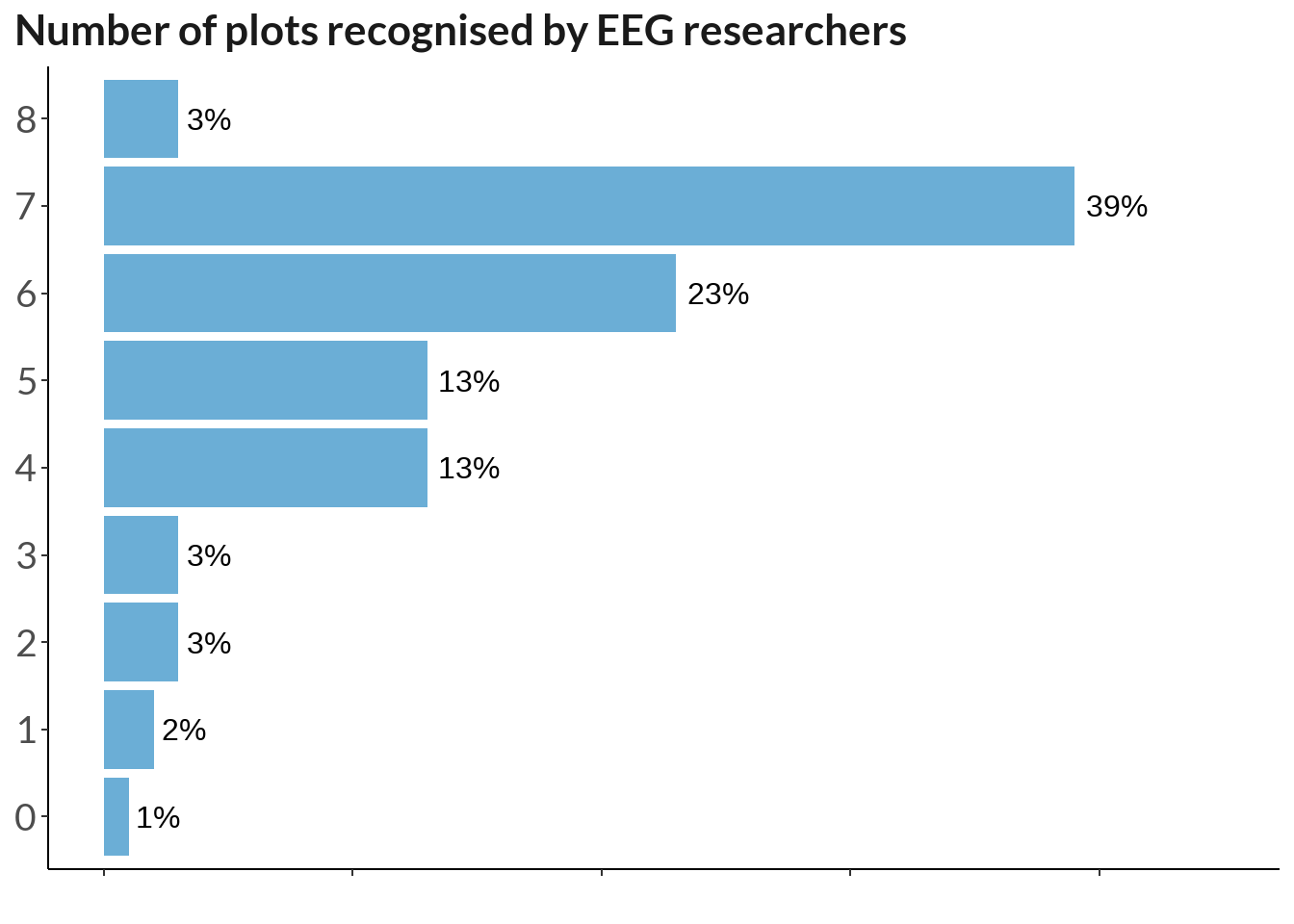 

Naming

Those who proposed a name for a plot. Bad names are excluded.

Code

stat_preproc <- function(vec){
  #N = 70
  tmp <- vec %>% filter(!is.na(.)) %>% 
    dplyr::rename(words = !!names(.)[1]) %>% mutate(words = tolower(words)) %>% 
    mutate(words = ifelse(nchar(words) < 3, paste(words, "baddd"), words)) %>% 
    mutate(check = 
    ifelse(grepl("\\b(baddd|idea|sure|confus|aware|do not|know|why|good|remember|unsure|confusing|mess|unclear|ugly|don't|useless|nan|clear)\\b", words), "bad", "good")) 
  return(tmp)
}

#stat_preproc(data[vec_named[7]]) %>% View()

Code

vec_named <- names(data[ , grepl( "How would you " , names(data))])
plot_names <- c("line", "butterfly", "topo", "topo_series", "erp_grid", "erp_img", "parallel", "channel_img")

na_table <- function(data, vec_named, plot_names){
    temp <- data.frame(plot_names)
    temp$n <- NA
    for (i in 1:8){
      n_part <- data[vec_named[i]] %>%  stat_preproc(.) %>% #View()
      filter(check != "bad") %>%  
      dplyr::summarise(n = n())  
      temp$n[i] <- n_part$n
    }
    return(temp)
}

num_named <- na_table(data, vec_named, plot_names)
num_named  %>% 
  ggplot(., aes(x = n, y = reorder(plot_names, n))) +
  geom_col(stat="identity",  fill ="#6BAED6") +
    labs(x = "Category", y = "Value") +
    theme_classic() + theme(axis.title.x=element_blank(), plot.title = element_text(hjust = 0.5)) +
  geom_text(aes(label = n), position = position_dodge(width = .9), hjust = -0.1) +
  ggtitle("Plot naming") +
  labs(caption = sprintf("N of respondents - %d",  nrow(familiar))) +
  theme(legend.position="none", plot.caption = element_text(hjust=0), axis.text = element_text(size = 10))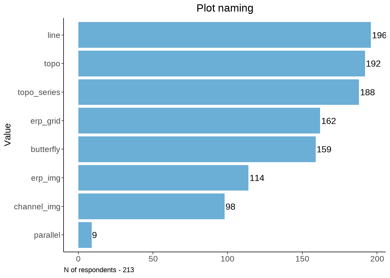

Code

tmp <- data[vec_named]
tmp$n <- rowSums(!is.na(tmp)) 
table(tmp$n)  %>%  t() %>% data.frame() %>% select(-Var1) %>% 
  mutate(percent_score = round(Freq / 213 * 100)) %>% 
  ggplot(., aes(y = Var2, x = percent_score)) +
  geom_col(stat="identity", fill ="#6BAED6") +
    labs(x = "", y = "Number of named plots", title = "Number of plots named by EEG researchers") + theme_classic() +
    geom_text(aes(label = paste0(percent_score, "%")), 
              position = position_dodge(width = .9), hjust = -0.2, size = 4) + theme(
      axis.text.y = element_text(size = 14),
      legend.position="none", plot.caption.position = "plot", 
      plot.caption = element_text(hjust=0), 
      text = element_text(family = "Lato"),
      axis.text.x = element_blank(), axis.text = element_text(size = 10),  
      plot.title = element_text(color = "grey10", size = 16, face = "bold"),
      axis.title.y = element_blank(),
      plot.title.position = "plot"
      ) + xlim(0, 39)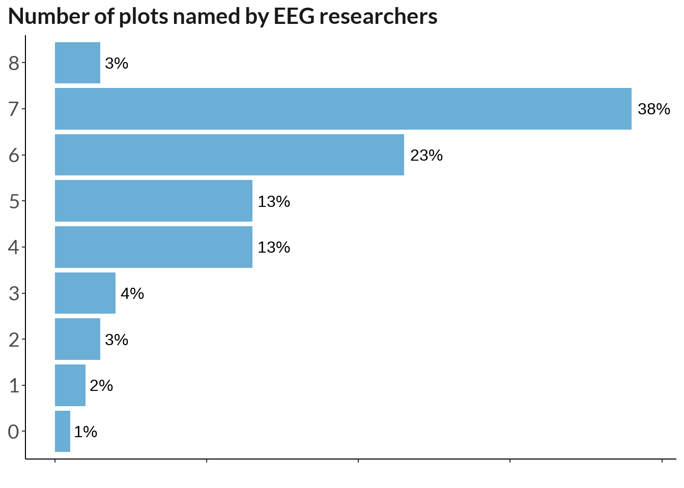 

Plotting

Code

familiar <-  data[61:68] %>% rename_at(vars(colnames(.)), ~ plot_names) %>% 
  mutate_at(vars(plot_names), function(., na.rm = FALSE) (x = ifelse(.=="Yes", 1, 0))) %>%
  t() %>% rowSums(.) %>% data.frame(.) %>%  tibble::rownames_to_column(., "plot") %>% 
  rename_at(vars(colnames(.)), ~ c("plots", "recognized"))

combined

Code

plot_vec <- rev(c("Parallel\nplot", "Channel\nimage", "ERP image", "Butterfly\nplot", "ERP grid", "Topoplot\ntimeseries", "Topoplot", "ERP plot"))

vec_plotted <- names(data[ , grepl( "Have you ever plotted " , names(data))]) 

do_vec <- function(vec_plotted, data, plot_names){
  t1 <- table(data[vec_plotted[1]])
  for (i in 2:length(vec_plotted)) {
    t <- table(data[vec_plotted[i]])
    t1 <- rbind(t1, t)
  }
  rownames(t1) <- plot_names 
  return(t1)
}

tab <- do_vec(vec_plotted, data, plot_names) %>%  data.frame() %>% tibble::rownames_to_column(., "plots") %>%  
  gather(., type, plotted, `N.A`:`Yes`, factor_key=TRUE) %>% 
  filter(type == "Yes") %>% dplyr::select(-type) 

named <- num_named %>% dplyr::rename(named = n, plots = plot_names)  

Code

mem_tab <-  familiar %>% 
   rename_at(vars(colnames(.)), ~ c("plots", "recognized")) %>%
  left_join(., named)  %>% left_join(., tab)  

mem_tab_fig <- mem_tab %>% 
  gather(., type, score,  recognized:plotted, factor_key=TRUE) %>% 
  ggplot(., aes(x = score, y = reorder(plots, -score), fill = reorder(type, score))) +
    geom_bar(position = "dodge", stat = "identity") +
    labs(y = "", x = "Number of users", title = "Level of familiarity with a plot") +
    theme_classic() + 
  geom_text(aes(label = score, group = reorder(type, score)), position = position_dodge(width = .9), hjust = -0.2, size = 3) +  
  xlim(0, 210) + 
  scale_fill_brewer(palette = "Blues") +
  guides(fill = guide_legend(reverse=T)) +
  scale_y_discrete(labels = plot_vec) +
  theme(plot.caption = element_text(hjust=0), 
        axis.text = element_text(size = 10), 
        text = element_text(family = "Lato"), 
        legend.title = element_blank(),
        legend.position = c(0.8, 0.9),
        plot.title = element_text(hjust = 0.5),
        axis.title = element_text(size = 12),
        plot.title.position = "plot") 

mem_tab_fig +
  labs(caption = sprintf("N of respondents - %d",  nrow(data[61:68])))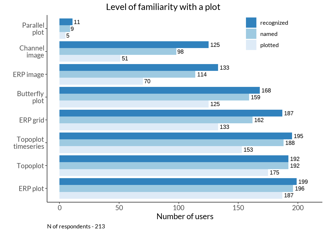

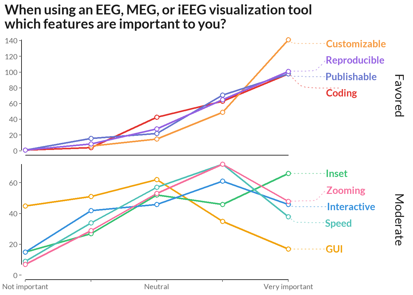
Important features

Code

feature <- data[52:60] %>% rename_all(., ~str_split_i(colnames(data[52:60]), "\\? \\[", 2) %>% str_sub(., 1, -2) ) %>%  
  mutate_at(c(colnames(.)), 
        funs(recode(.,
        "Very important"= 2, "Important"= 1, "Neutral"= 0,
        "Low importance"= -1, "Not at all important" = -2 )))

feature %>% 
  colSums(., na.rm =T) %>% data.frame(.) %>%  tibble::rownames_to_column(., "Feature") %>% 
  filter(!is.na(Feature)) %>% 
  arrange(desc(.)) %>% rename_at(vars(colnames(.)), ~ c("Feature", "sum_scores")) %>% group_by(Feature) %>% 
  dplyr::mutate( mean = round(sum_scores / nrow(data), 2)) %>%   kbl(escape = F, booktabs = T) %>%
  kable_styling("striped", position = "center",) %>% kable_classic(full_width = F, html_font = "Arial")

Feature	sum_scores	mean
Flexible tweaking of plot attributes (colors, linewidths, margins etc.)	325	1.53
Reproducibility of interactively generated or modified plots	256	1.20
Generating plots by coding	253	1.19
Presentation/publication ready figures	249	1.17
Zooming or panning within a plot	125	0.59
Combine with a custom plot created outside of the toolbox (as subplot or inset)	121	0.57
Speed of plotting	96	0.45
Interactive selection of time-ranges or electrodes e.g. via Sliders or Dropdown menus	81	0.38
Generating plots by clicking (GUI)	-72	-0.34

Code

feature1 <- feature %>% 
  pivot_longer(cols = everything(), names_to = "name", values_to = "value") %>% 
  mutate(index = as.integer(factor(name))) %>% 
  filter(!is.na(value))

Code

plot_features <- c(
  "Combine with a custom plot created outside of the toolbox (as subplot or inset)",
  "Flexible tweaking of plot attributes (colors, linewidths, margins etc.)",
  "Speed of plotting",
  "Presentation/publication ready figures",
  "Reproducibility of interactively generated or modified plots",
  "Zooming or panning within a plot",
  "Interactive selection of time-ranges or electrodes e.g. via Sliders or Dropdown menus",
  "Generating plots by clicking (GUI)",
  "Generating plots by coding"
)

comb_data <- feature1 %>%  mutate(name = case_when(
  name == "Combine with a custom plot created outside of the toolbox (as subplot or inset)" ~ "Inset",
  name == "Flexible tweaking of plot attributes (colors, linewidths, margins etc.)"~ "Customizable",
  name == "Speed of plotting"~ "Speed",
  name == "Presentation/publication ready figures"~ "Publishable",
  name == "Reproducibility of interactively generated or modified plots"~ "Reproducible",
  name == "Zooming or panning within a plot"~ "Zooming",
  name == "Interactive selection of time-ranges or electrodes e.g. via Sliders or Dropdown menus"~ "Interactive",
  name == "Generating plots by clicking (GUI)"~ "GUI",
  name == "Generating plots by coding" ~ "Coding"
  )) %>% 
    mutate(gr = case_when(
      grepl("\\b(Speed|Zooming|GUI|Interactive)\\b", name) == TRUE ~ "Moderate",
      grepl("\\b(Coding|Customizable|Reproducible|Publishable|Inset)\\b", name) == TRUE ~ "Favored"))

test <-  comb_data %>% group_by(name, value) %>% dplyr::summarise(n = n()) %>% 
    mutate(gr = case_when(
      grepl("\\b(Speed|Zooming|GUI|Interactive|Inset)\\b", name) == TRUE ~ "Moderate",
      grepl("\\b(Coding|Customizable|Reproducible|Publishable)\\b", name) == TRUE ~ "Favored"))  %>% 
  mutate(denymax = case_when(value == 2 ~ n, TRUE ~ NA))

cbPalette_fe <- c("#e3342f", "#f6993f", "#f1a20b", "#38c172", "#3490dc", "#6574cd", "#9561e2", "#4dc0b5", "#f66d9b")

Code

test %>%  
  ggplot(aes(x = value, y = n, label = name, full = name)) + 
   geom_col(stat = "identity", bw = 0.5, size = 1) + facet_wrap(~name)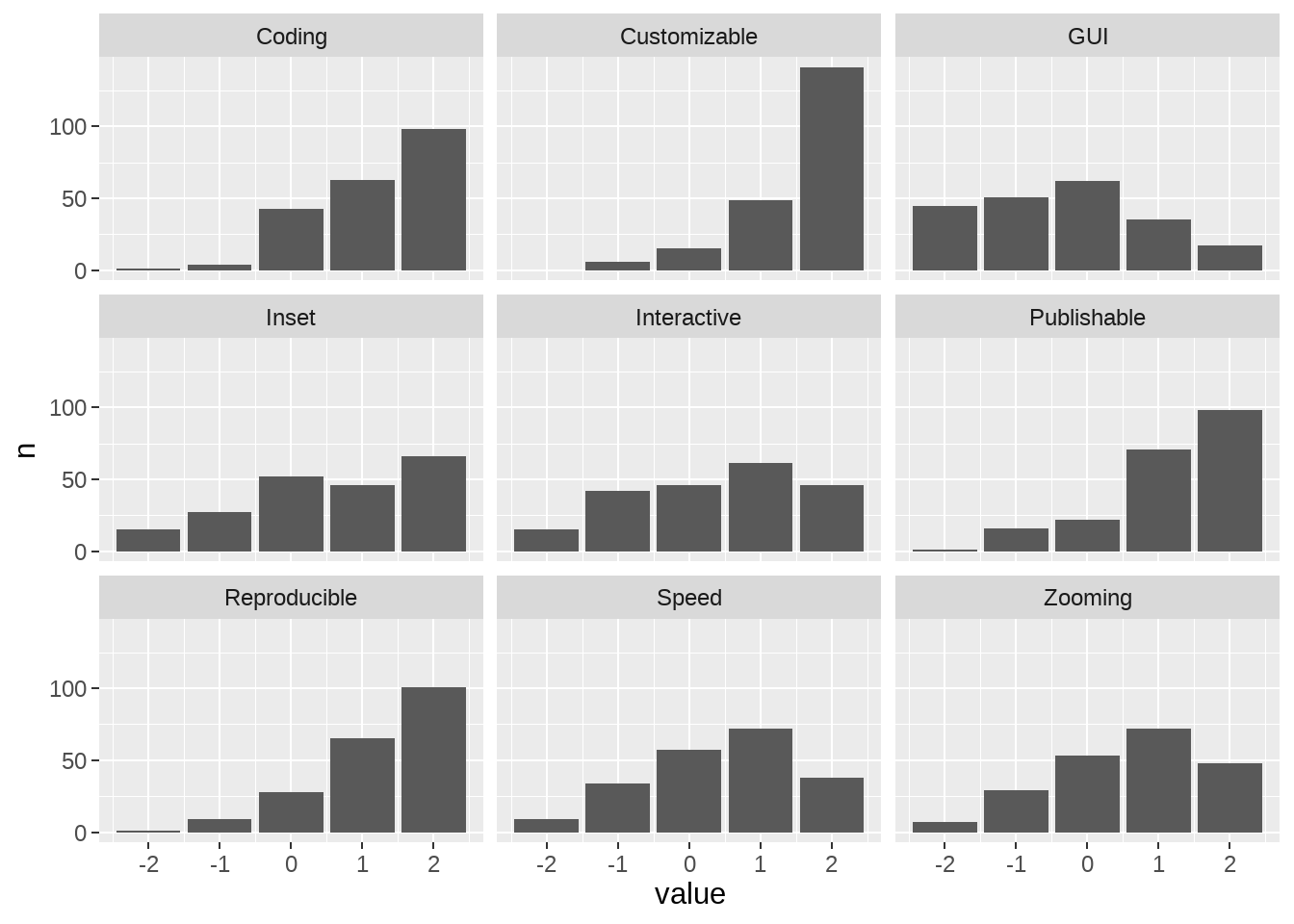

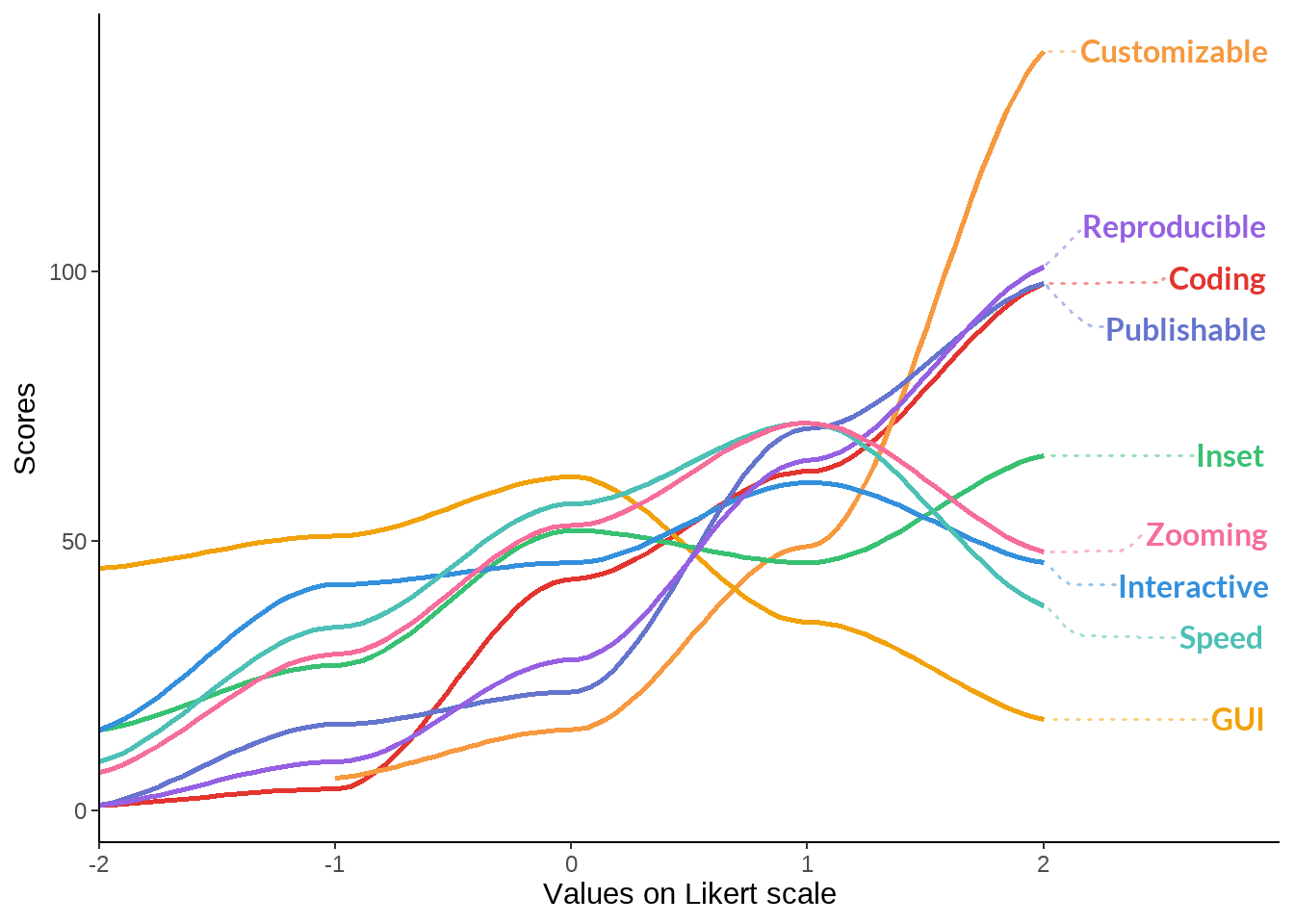
Code

test  %>% 
  ggplot(aes(x = value, y = n, label = name, color = name)) + 
   geom_smooth(aes(x = value, y = n),  size = 1) + #facet_wrap(~gr) +  
  scale_color_manual(values=cbPalette_fe) + theme_classic()  +  
  theme(legend.position = "none", 
  strip.background = element_blank(), 
  strip.text = element_text(size = 14),
) + labs(x = "Values on Likert scale", y = "Scores") +
  geom_text_repel(
    aes(color = name, label = name, x = 2, y = denymax,),
    family = "Lato",
    fontface = "bold",
    size = 4,
    direction = "y",
    xlim = c(3, NA),
    hjust = 0,
    segment.size = .7,
    segment.alpha = .5,
    segment.linetype = "dotted",
    box.padding = .4,
    segment.curvature = -0.1,
    segment.ncp = 3,
    segment.angle = 20
  ) +
  scale_x_continuous(
    expand = c(0, 0),
    limits = c(-2, 3), 
    breaks = seq(-2, 2, by = 1)
  )

Code

test  %>% mutate(value = value + 3) %>% 
  ggplot(aes(x = value, y = n, label = name, color = name)) + 
  geom_line(bw = 0.5, size = 1) + 
  geom_point(shape = 21, fill = 'white', size=2, stroke=1) + 
  facet_grid(gr~ ., scales = "free_y") +  
  scale_color_manual(values = cbPalette_fe) + 
  labs(x = "Values on the Likert scale", y = "Scores")  +  geom_rangeframe(color = "black") +
  theme(
    panel.background = element_blank(), panel.border = element_blank(), 
    legend.position = "none", 
    text = element_text(family = "Lato"),
    strip.background = element_blank(), 
    #axis.line.x =  element_blank(),
    axis.text = element_text(color = "grey40"),
    axis.ticks = element_line(color = "grey40", size = .5),
    strip.text = element_text(size = 14),
    axis.title = element_blank(),
    plot.title = element_text(
      color = "grey10", 
      size = 16, 
      face = "bold",
      #margin = margin(t = 15)
      ),
    plot.title.position = "plot",
  )  + 
  scale_x_continuous(
    expand = c(0.01, 0),
    limits = c(0.9, 5), 
    breaks = seq(1, 5, by = 1),
    labels = c("Not important", "", "Neutral", "", "Very important")
  ) +
  scale_y_continuous(
    expand = c(0.04, 0),
    limits = c(0, NA),
    breaks = seq(0, 150, by = 20)
  ) +
  labs(title = "When using an EEG, MEG, or iEEG visualization tool\nwhich features are important to you?")   +
  coord_cartesian(xlim = c(1, 6.5), clip = "off") +
  geom_text_repel(
    aes(color = name, label = name, x = 5, y = denymax,),
    family = "Lato",
    fontface = "bold",
    size = 4,
    direction = "y",
    xlim = c(5.5, NA),
    hjust = 0,
    segment.size = .7,
    segment.alpha = .5,
    segment.linetype = "dotted",
    box.padding = .4,
    segment.curvature = -0.1,
    segment.ncp = 3,
    segment.angle = 20
  )

Code

cbPalette_fe1 <- c("#e3342f", "#6574cd", "#f6993f",  "#38c172" )

cbPalette_fe2 <- c("#4dc0b5", "#3490dc","#f1a20b", "#9561e2", "white", "#f66d9b")
core <- function(df){
  g <- ggplot(data = df, aes(x = value, y = n, label = name, color = name)) + 
  geom_line(bw = 0.5, size = 1) + 
  geom_point(shape = 21, fill = 'white', size=2, stroke=1)+ 
  labs(x = "Values on the Likert scale", y = "Scores")  +  geom_rangeframe(color = "black") +
  theme(
    panel.background = element_blank(), panel.border = element_blank(), 
    legend.position = "none", 
    text = element_text(family = "Lato"),
    strip.background = element_blank(), 
    axis.text = element_text(color = "grey40"),
    axis.ticks = element_line(color = "grey40", size = .5),
    strip.text = element_text(size = 14),
    axis.title = element_blank(),
    plot.title = element_text(
      color = "grey10", 
      size = 16, 
      face = "bold",
      ),
    plot.title.position = "plot",
  )  +
  coord_cartesian(xlim = c(1, 6.5), clip = "off") +
  geom_text_repel(
    aes(color = name, label = name, x = 5, y = denymax,),
    family = "Lato",
    fontface = "bold",
    size = 4,
    direction = "y",
    xlim = c(5.5, NA),
    hjust = 0,
    segment.size = .7,
    segment.alpha = .5,
    segment.linetype = "dotted",
    box.padding = .4,
    segment.curvature = -0.1,
    segment.ncp = 3,
    segment.angle = 20
  ) 
  return(g)
} 

test1 <- test %>% filter(gr == "Favored") %>% mutate(value = value + 3) %>% 
  core(.) +
  scale_x_continuous(
    expand = c(0.01, 0),
    limits = c(0.9, 5), 
    breaks = seq(1, 5, by = 1)
  ) +
  scale_y_continuous(
    expand = c(0.04, 0),
    limits = c(0, NA),
    breaks = seq(0, 150, by = 30)
  ) +
  scale_color_manual(values = cbPalette_fe1) + theme(axis.text.x=element_blank()) +
  labs(title = "When using an EEG, MEG, or iEEG visualization tool\nwhich features are important to you?")  


test2 <- test %>% filter(gr != "Favored") %>% mutate(value = value + 3) %>% ungroup() %>% 
  tibble::add_row(name = "void", value = 1, n = 0, gr = "a", denymax=0) %>% 
  # line above is just to extend yaxis to zero
   core(.) +
  scale_x_continuous(
    expand = c(0.01, 0),
    limits = c(0.9, 5), 
    breaks = seq(1, 5, by = 1),
    
    labels = c("Not important", "", "Neutral", "", "Very important")
  ) +
  scale_y_continuous(
    expand = c(0.04, 0),
    limits = c(0, NA),
    breaks = seq(0, 72, by = 15)
  ) + 
  scale_color_manual(values = cbPalette_fe2) + theme(axis.text.x = element_text(color = "black"))

figure <- ggarrange(test1, test2, align = 'v', nrow = 2) 
require(grid)
annotate_figure(figure, left = textGrob("Number of responses", rot = 90, vjust = 1, gp = gpar(cex = 1.3)))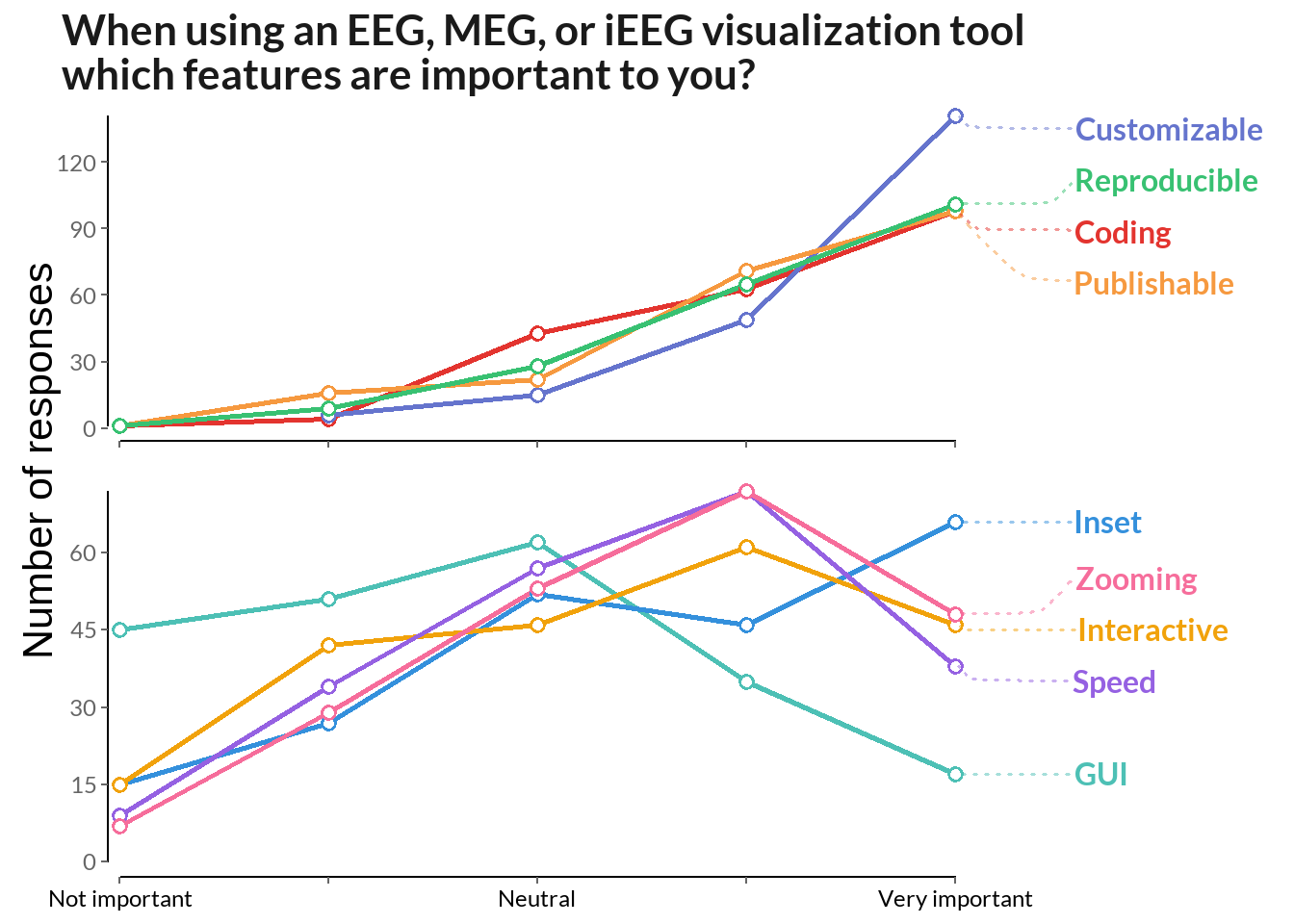

Controversies

Channels

How many channels do you typically analyse and measure?

Code

cv <- data %>% select(23, 24) %>% 
  rename_at(vars(colnames(.)), ~ c("measure", "analyse")) %>% 
  filter(measure < 10000, analyse < 500)  %>% 
  mutate(rate = round(analyse / measure, 2)) %>% 
  group_by(rate) %>% dplyr::summarise(n = n()) %>% 
  mutate(p = round(n / sum(n), 2))

an_me_plot <- cv %>%  
  ggplot(aes(x=rate, y = p)) + 
  geom_col(position = "identity", bins=300, fill ="#6BAED6") + 
  labs(x ="Ratio of electrodes\nanalysed / measured", y = "") +
  theme_classic() +
  theme(legend.position="none", plot.caption = element_text(hjust=0), text = element_text(family = "Lato"), axis.text = element_text(size = 10)) + 
  #ylim(0, 0.1) + 
  scale_x_continuous(labels = scales::percent)  + scale_y_continuous(labels = scales::percent, limits = c(0, 0.4)) +
   labs(y = "Percent of respondents")

an_me_plot +
  labs(caption = sprintf("N of respondents - %d",  sum(cv$n)))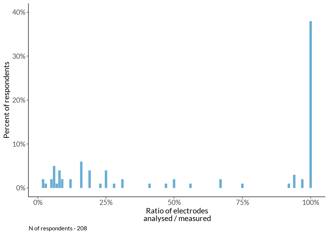 

Code

marg <- data %>% select(23, 24) %>% 
  rename_at(vars(colnames(.)), ~ c("Recorded", "Analysed")) %>% 
  filter(Recorded < 10000, Analysed < 500)   %>%  
  ggplot(., aes(y=Analysed, x = Recorded)) + geom_point() +
      theme(legend.position="none") + theme_classic() + labs(x = "Electrodes recorded", y = "Electrodes aanlysed")
ggMarginal(marg, type="histogram")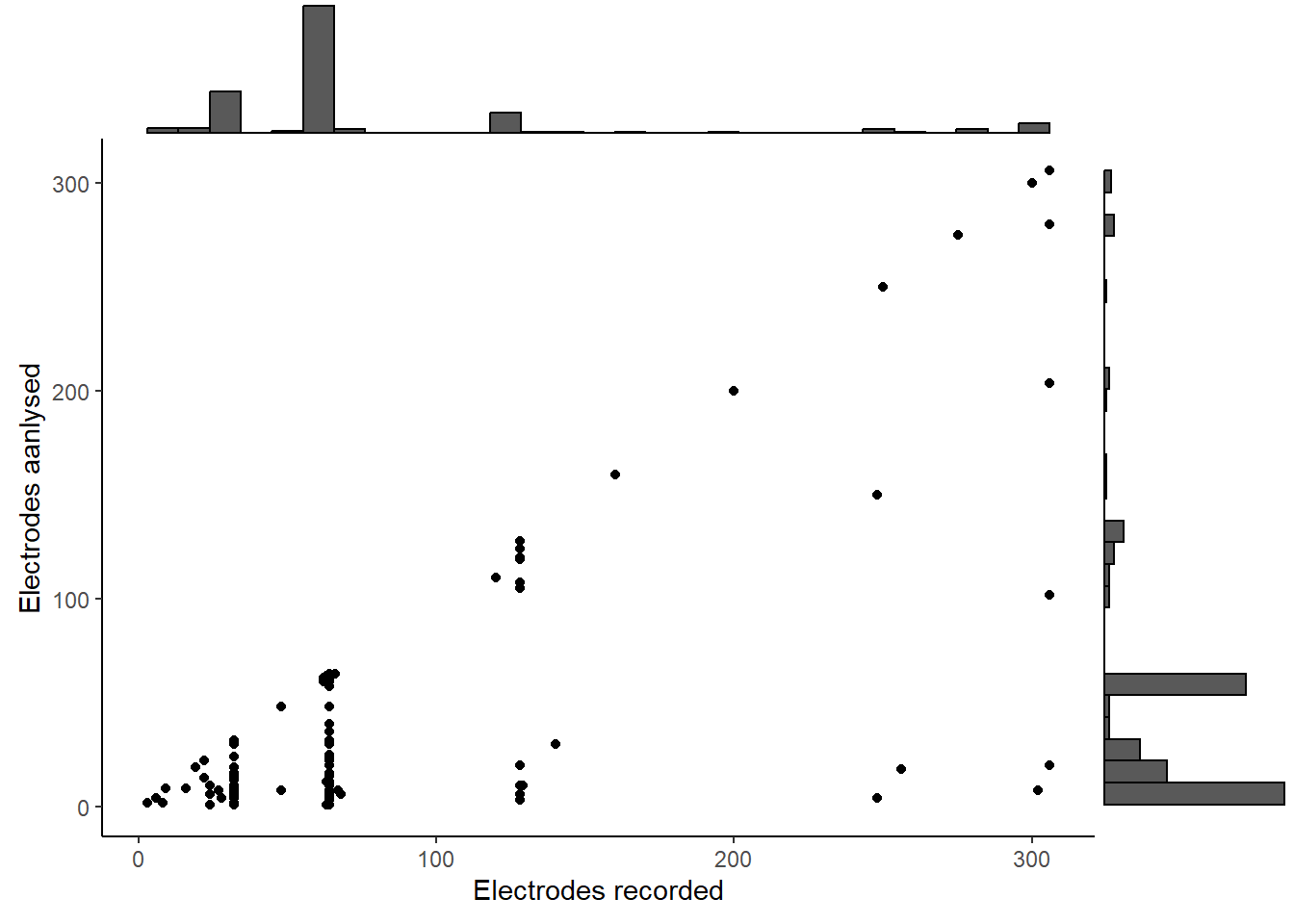

Up or down

Code

t <- foreach(i = 1:nrow(data)) %do% tokenize_words(as.character(data[i, 11]))
tt <- foreach(i = 1:length(t)) %do% paste(unlist(t[i]), collapse = ' ') 

area1 <- data.frame(matrix(tt)) %>% dplyr::rename(words = !!names(.)[1]) %>%
  mutate(words = ifelse(str_detect(.[[1]], 'emot|empathy'), "affective neuroscience", words)) %>%  
  mutate(words =ifelse(str_detect(.[[1]], 'memory'), "memory", words)) %>% 
  mutate(words =ifelse(str_detect(.[[1]], 'hearing|audit'), "auditory", words)) %>% 
  mutate(words =ifelse(str_detect(.[[1]], 'cognitive load|selective attention|attention|cognition|consciousness|meditation|cognitive control|self|executive functions'), "attention", words)) %>% 
  mutate(words =ifelse(str_detect(.[[1]], 'dbs'), "deep brain stimulation", words)) %>% 
  mutate(words =ifelse(str_detect(.[[1]], 'decision making|reward'), "decision making", words)) %>%
  mutate(words =ifelse(str_detect(.[[1]], 'ageing'), "ageing", words)) %>% 
  mutate(words =ifelse(str_detect(.[[1]], 'social'), "social cognition", words)) %>% 
  mutate(words =ifelse(str_detect(.[[1]], 'olfac'), "olfaction", words)) %>% 
  mutate(words =ifelse(str_detect(.[[1]], 'communication|language|speech|biling|english|language processing'), "language and speech", words)) %>% 
  mutate(words =ifelse(str_detect(.[[1]], 'bci'), "bci", words)) %>% 
  mutate(words =ifelse(str_detect(.[[1]], 'sleep'), "sleep", words)) %>% 
  mutate(words =ifelse(str_detect(.[[1]], 'timing|time|temporal'), "time", words)) %>% 
  mutate(words =ifelse(str_detect(.[[1]], 'perception'), "perception", words)) %>% 
  mutate(words =ifelse(str_detect(.[[1]], 'vis'), "vision", words)) %>% 
  mutate(words =ifelse(str_detect(.[[1]], 'developmental|development|ageing'), "development", words)) %>% 
  mutate(words =ifelse(str_detect(.[[1]], 'spatial|brain body|motor|motion'), "motor control", words)) %>% 
  mutate(words =ifelse(str_detect(.[[1]], 'diagnostics|disorder|psychiatry|epilepsy|autism|patients|therapy|psychopharmacology'), "mental disorders", words)) %>%   
  mutate(words =ifelse(str_detect(.[[1]], 'signal processing|event related potentials|method|sdf|ieeg'), "dsp", words))

area <- area1 %>%
  mutate(words = ifelse(str_detect(.[[1]], 'olfaction|vision|auditory|pain'), "perception", words))%>%
  mutate(words = ifelse(str_detect(.[[1]], 'dsp|computational neuroscience'), "methodology", words)) %>% 
  mutate(words = ifelse(str_detect(.[[1]], 'mental disorders|deep brain stimulation'), "clinical", words))%>% 
  mutate(words = ifelse(str_detect(.[[1]], 'social cognition'), "affective neuroscience", words))

Code

colours = c("#f9a65a", "#599ad3")
ud <- table(data[79]) %>% data.frame() %>% 
  rename_at(vars(colnames(.)), ~ c("position", "scores")) %>%
  mutate(percent_score = round(scores / sum(scores) * 100)) 

pol_not_plot1 <- ud %>% 
    ggplot(., aes(y = position, x = percent_score)) + #, fill = as.factor(percent_score))) +
    geom_bar(position = "dodge", stat = "identity", width=0.5, fill ="lightblue1", colour ="dodgerblue3") + 
    theme_classic() +
    theme(axis.title=element_blank(), 
          legend.position="none", axis.text.x = element_blank(),
          axis.text = element_text(size = 12),
          plot.title = element_text(hjust = 0.5)) +
  geom_text(aes(label = paste0(percent_score, "%"), group = position), hjust = -0.2) +
  ggtitle("In ERP plot, should positive voltages be plotted upwards, or downwards?") +
  scale_fill_manual(values=colours) + xlim(0, 83) +
    theme(legend.position="none", plot.caption = element_text(hjust=0), axis.text = element_text(size = 10))  

pol_not_plot1 +
    labs(caption = sprintf("N of respondents - %d",  sum(ud$scores)))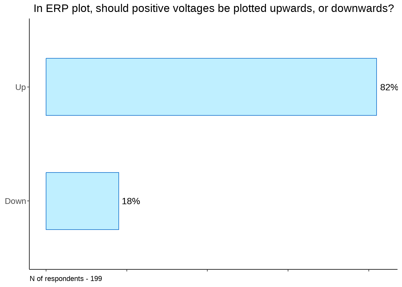 

Code

as <- cbind(unlist(area$words), unlist(data[[79]])) %>% data.frame() %>% 
filter(.[[2]] != "NANA") %>% dplyr::rename(area=X1, ud=X2) %>%
group_by(area) %>%
filter(n() > 2) %>% group_by(area, ud) %>% dplyr::summarise(n = n()) %>% 
  group_by(area) %>% dplyr::mutate(nn = sum(n)) %>% filter(area != "")

pol_not_plot2 <- as %>% 
  ggplot(., aes(x = n, y = reorder(area, nn), fill = ud)) +
  geom_col(stat = "identity", width = 0.7) +
  labs(x = "Percent of respondents", y = "", fill ="Positive:", title = "In ERP plot, should positive voltages\nbe plotted upwards, or downwards?") +
  theme_classic()+
  geom_text(aes(label = n, group = ud), 
            position = position_stack(vjust = 0.5), size = 4)  +
  coord_cartesian(clip = "off") +
  theme(axis.text = element_text(size = 12),
        text = element_text(family = "Lato"),
        axis.title = element_text(size = 12),
        title = element_text(size = 14),
        axis.title.y=element_blank(),
        
        legend.title = element_blank(),
        legend.direction = "horizontal",
        legend.position = c(0.8, 0.2),
        
        plot.title.position = "plot",
        plot.caption.position = "plot",
        ) +  
  scale_fill_manual(values=colours, limits = c("Up", "Down")) 

pol_not_plot2 +
    labs(caption = sprintf("N of respondents - %d",  sum(as$n)))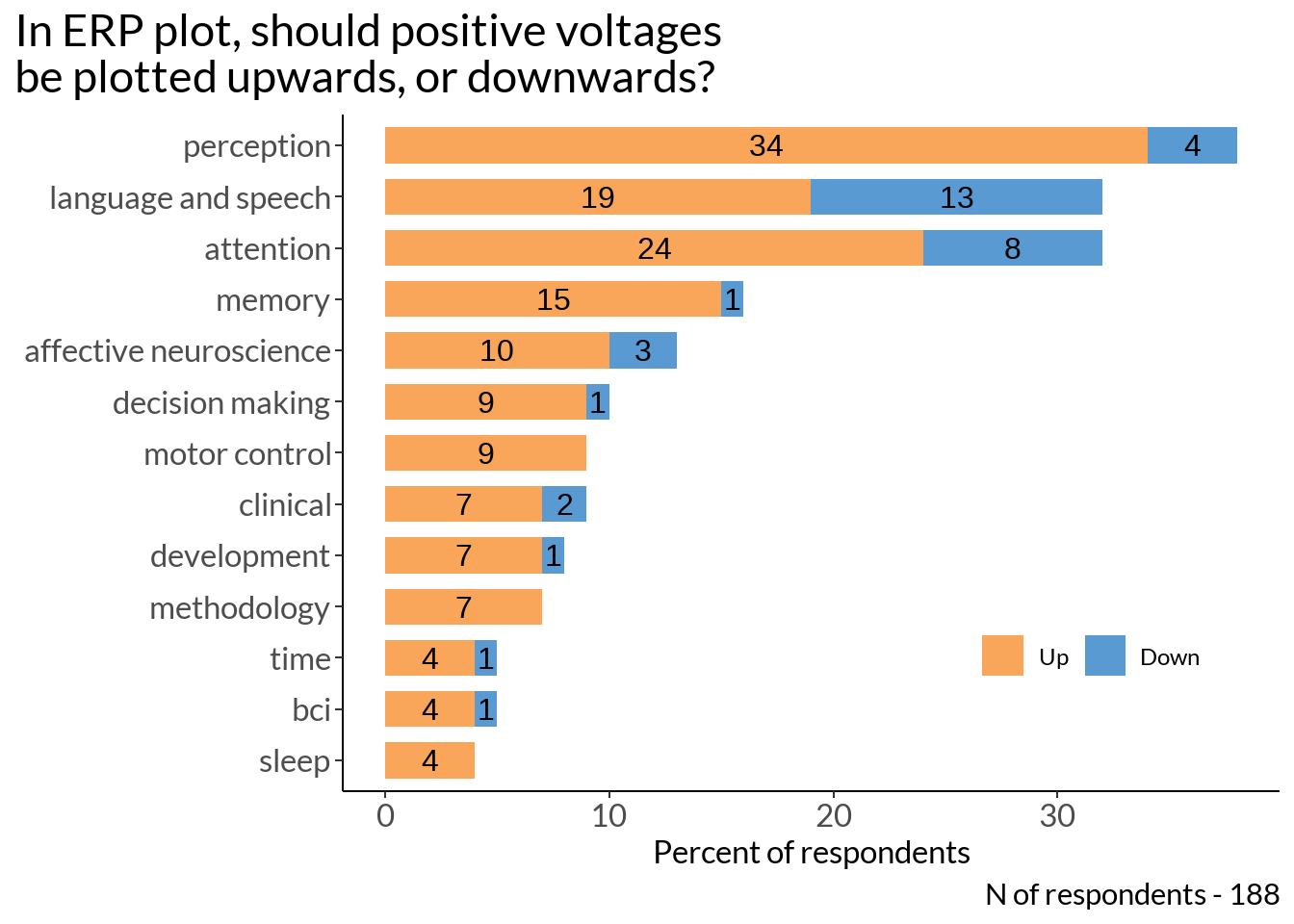

Code

area_short <- area %>% 
  mutate(words = ifelse(str_detect(.[[1]], 'language and speech|attention'), 
                        "language, speech,
                        attention", 
                        "affective neuroscience,\nbci, clinical, decision making,\ndevelopment, memory,\nmethodology, motor control,\nperception, sleep, time")) 

as2 <- cbind(unlist(area_short$words), unlist(data[[79]])) %>% data.frame() %>% 
filter(.[[2]] != "NANA") %>% dplyr::rename(area=X1, ud=X2) %>%
group_by(area) %>%
filter(n() > 2) %>% group_by(area, ud) %>% dplyr::summarise(n = n()) %>% 
  group_by(area) %>% dplyr::mutate(nn = sum(n)) %>% filter(area != "")

pol_not_plot3 <- as2 %>% 
  ggplot(., aes(x = n, y = reorder(area, nn), fill = ud)) +
  geom_col(stat = "identity", width = 0.7) +
  labs(x = "Percent of respondents", y = "", fill ="Positive:", title = "In ERP plot, should positive voltages\nbe plotted upwards, or downwards?") +
  theme_classic()+
  geom_text(aes(label = n, group = ud), 
            position = position_stack(vjust = 0.5), size = 4)  +
  coord_cartesian(clip = "off") +
  theme(axis.text = element_text(size = 12),
        text = element_text(family = "Lato"),
        axis.title = element_text(size = 12),
        title = element_text(size = 14),
        axis.title.y=element_blank(),
        
        legend.title = element_blank(),
        legend.direction = "horizontal",
        legend.position = c(0.8, 0.2),
        
        plot.title.position = "plot",
        plot.caption.position = "plot",
        ) +  
  scale_fill_manual(values=colours, limits = c("Up", "Down")) 

pol_not_plot3 +
    labs(caption = sprintf("N of respondents - %d",  sum(as$n)))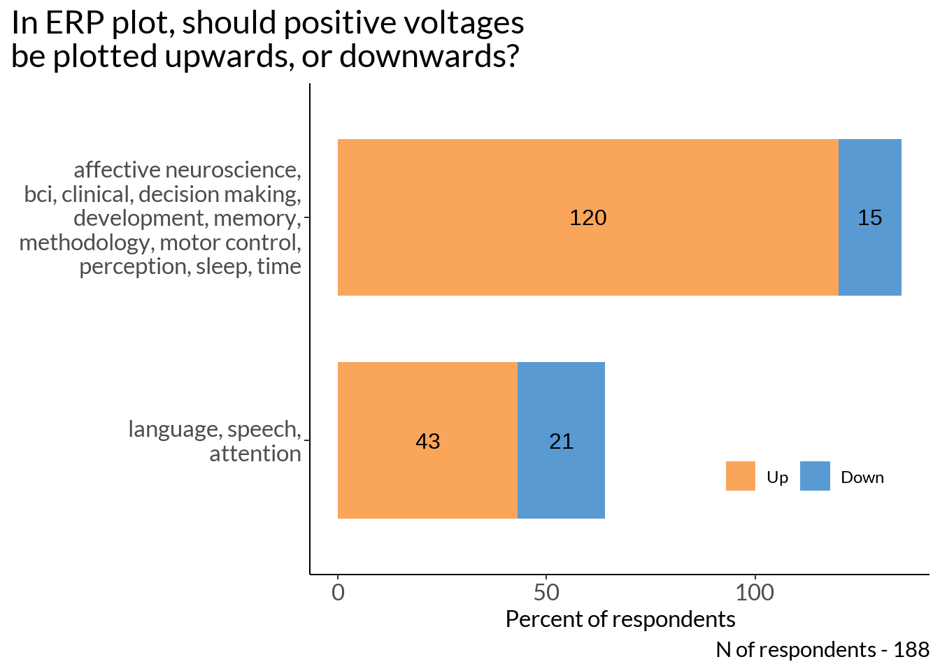

Baseline

Think about the baseline period (the time before the stimulus onset). How many milliseconds would you recommend to plot? Help: Please, provide the baseline duration for the plot, not the duration for the baseline-correction

justification

Code

# If you don't want to provide a number on previous question, please, provide a justification
j <- data %>%    
  dplyr::rename(q = !!names(.)[78]) %>% filter(!is.na(q)) %>% dplyr::select(q) %>% 
  mutate(q = tolower(q)) %>% mutate(q = gsub('depends in|depending on', 'depends on', q),
         dependson = ifelse(grepl("depends|depend", q), q, NA)) %>% 
  separate(dependson, into = c("a","b"), sep = "depends on |depend on ") %>% 
  dplyr::select(-a) %>% 
  dplyr::rename(dependson = b) #%>% 
j %>% filter(!is.na(dependson)) %>% select(dependson)

# A tibble: 37 × 1
   dependson                                                                    
   <chr>                                                                        
 1 "the design of course"                                                       
 2 "the topic"                                                                  
 3 "the study. if you have interstimulus interval of 1 second and you expect to…
 4 "the experiment and research question"                                       
 5 "the rest period between the measured evoked responses. e.g. it can be very …
 6 "the analysis"                                                               
 7 "paradigm, 100-300 ms range preferable"                                      
 8 "the task design"                                                            
 9 "the type of response (eg for mrcps response is seen before actual movement …
10 "the task design, paradigm and signal of interest."                          
# ℹ 27 more rows

Code

j %>% filter(is.na(dependson))  %>% select(-dependson)

# A tibble: 21 × 1
   q                                                                            
   <chr>                                                                        
 1 minimum 200ms for erps and theta or beta power                               
 2 should match the duration of baseline-correction                             
 3 as a rule of thumb, i would plot at least 1/3 of the duration (post-stimulus…
 4 half of the illustrated task interval                                        
 5 in general i would always try to plot the full baseline period used for base…
 6 the same duration as the one used for baseline correction                    
 7 at least 300, preferably more                                                
 8 put down 100, but that's just what i typically use, might be diff for differ…
 9 at least the baseline window used for the baseline correction?               
10 in this case it has sense as the -100 : 0 ms is not flat                     
# ℹ 11 more rows

Code

#j %>% write.csv(., "../data/justification.csv")

just <- read.csv("../data/justification.csv") %>% dplyr::select(group, num)

just2 <- just %>% filter(is.na(num)) %>% group_by(group) %>% dplyr::summarise(n = n())

periods

Code

bl <- table(abs(just[2] %>% na.omit() %>% rbind(data[77] %>% dplyr::rename(num = !!names(.)[1]) , .))) %>% data.frame() %>%  dplyr::rename(baseline = !!names(.)[1]) %>% 
  mutate(percent_score = round(Freq / sum(Freq), 2) *100)

periods_plot <- bl %>%
    ggplot(data = ., aes(x = baseline, y = percent_score)) +
    geom_bar(stat="identity", fill ="lightblue1", colour ="dodgerblue3") + 
  labs(x = "Recomended baseline duration in msec", y = "") +  
  scale_y_continuous(breaks=seq(0, 60, 5)) + theme_classic() +
  theme(legend.position="none", plot.title = element_text(hjust = 0.5), text = element_text(family = "Lato")) +
  geom_text(aes(label = paste0(percent_score, "%"), group = baseline), position = position_dodge(width = .9), vjust = -0.3)   +
    theme(legend.position="none", plot.caption = element_text(hjust=0), axis.text.y = element_blank(), axis.text = element_text(size = 10))

periods_plot +
    labs(caption = sprintf("N of respondents - %d",  sum(bl$Freq)))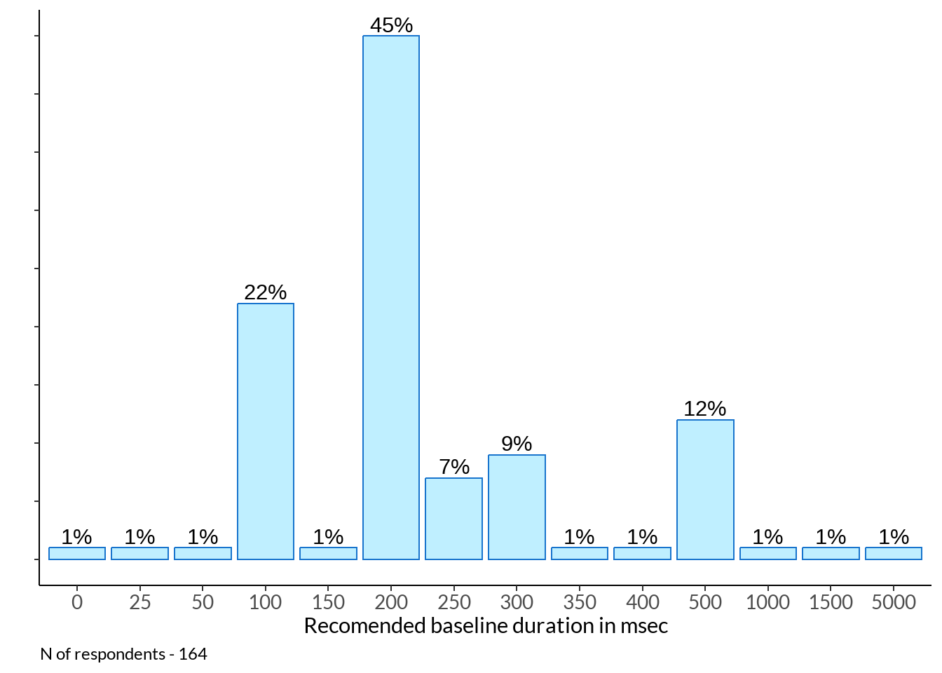

Code

bl2 <- table(abs(just[2] %>% na.omit() %>% rbind(data[77] %>% dplyr::rename(num = !!names(.)[1]) , .))) %>% data.frame() %>%  dplyr::rename(baseline = !!names(.)[1]) %>% 
  mutate(baseline = ifelse(Freq > 2, paste0("-", as.character(baseline)), "Other")) %>%
  dplyr::group_by(baseline) %>% dplyr::summarise(Freq = sum(Freq)) %>% 
  mutate(percent_score = round(Freq / sum(Freq), 2) *100) %>% arrange(desc(baseline)) %>% 
  mutate(baseline = factor(baseline, 
  levels = c("-500", "-300", "-250", "-200", "-100", "Other")))

italised1 <- c("-500", "-300", "-250", "-200", "-100", expression(italic("Other")))

periods_plot2 <- bl2 %>%
    ggplot(data = ., aes(x = baseline, y = percent_score)) +
    geom_bar(stat="identity", fill ="#6BAED6", width = 0.6) + 
  labs(x = "Recomended baseline duration\n(msec)", y = "") +  
  scale_y_continuous(breaks=seq(0, 60, 5)) + theme_classic() +
  theme(legend.position="none", plot.title = element_text(hjust = 0.5), text = element_text(family = "Lato")) +
  geom_text(aes(label = paste0(percent_score, "%"), group = baseline), position = position_dodge(width = .9), vjust = -0.3)   +
    theme(legend.position="none", plot.caption = element_text(hjust=0), axis.text.y = element_blank(), axis.text = element_text(size = 10)) + 
  scale_x_discrete(labels = italised1)

periods_plot2 +
    labs(caption = sprintf("N of respondents - %d",  sum(bl$Freq)))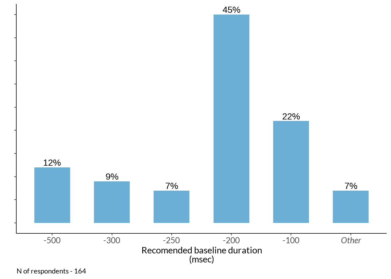

Topoplot timeseries interpretation

Code

tti_data <- data[95] %>% rename_at(vars(colnames(.)), ~ c("toposeries_int")) %>% filter(!is.na(.), toposeries_int != "Other") %>%
  group_by(toposeries_int) %>% dplyr::summarise(n = n()) %>% mutate(toposeries_int = case_when(
  toposeries_int == "The instantaneous time slices (single time points)" ~ "Time point",
  toposeries_int == "The mean value of time bin, centered around the labelled time (average over multiple time points)"~ "Average over\ntime points"
  )) %>% mutate(p = round(n / sum(n) * 100)) 

tti <-  tti_data %>% ggplot(., aes(y = toposeries_int, x = p)) + 
    geom_bar(stat = "identity", width=0.5, position = "dodge", fill ="#6BAED6") + theme_classic() +
    theme(
      text = element_text(family = "Lato"),
      legend.position="none", 
      strip.background = element_blank(), 
      axis.ticks = element_line(color = "grey40", size = .5),
      axis.text.x = element_blank(),
      axis.text.y =  element_text(color = "grey10", size = 16),
      axis.title.x=element_blank(), 
      plot.title = element_text(color = "grey10", size = 18, face = "bold", margin = margin(t = 15)),
      plot.title.position = "plot",
      plot.caption = element_text(hjust=0), 
    ) +
  geom_text(aes(label = paste0(p, "%"), group = toposeries_int), hjust = -0.2, size = 5, family = "Lato") + 
  labs(title = "How do you interpret time in topoplot timeseries?", subtitle = "", y = "")+
  scale_fill_manual(values=colours)  +
  xlim(0, 100)

tti  +
    labs(caption = sprintf("N of respondents - %d",  sum(tti_data$n))) # change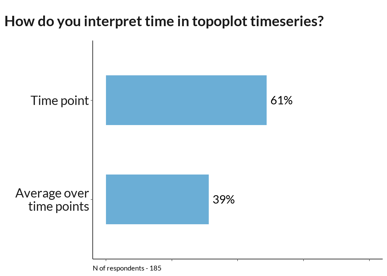

Combined

Code

ggarrange(periods_plot2 + labs(y = "Percent of respondents")+ theme(axis.title.y = element_text(margin = margin (r = 10))), 
          an_me_plot + theme(axis.title.y = element_text(margin = margin (r = 10))), labels = c("A", "B"))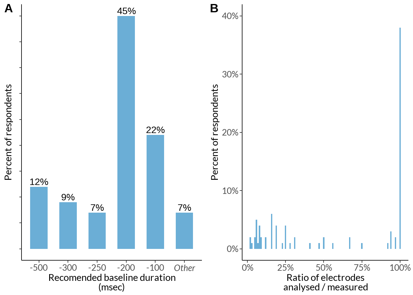 

Code

ggarrange(pol_not_plot2, tti, labels = c("A", "B"))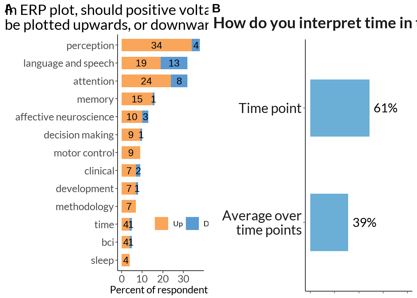

Awareness

Error bars

Code

table(data[74]) %>% data.frame() %>% rename_at(vars(colnames(.)), ~ c("position", "Scores"))  %>% 
  filter(position != "Never published this plot") %>% mutate(sum = sum(Scores)) 

  position Scores sum
1       No     63 157
2      Yes     94 157

Code

table(data[74]) %>% data.frame() %>% rename_at(vars(colnames(.)), ~ c("position", "Scores"))   %>%  mutate(percent_score = round(Scores / sum(Scores) * 100)) %>% 

    ggplot(., aes(x = position, y = percent_score, fill = as.factor(percent_score))) +
    geom_bar(position = "dodge", stat = "identity", width=0.5) + theme_classic() +
  theme(axis.title.x=element_blank(), 
        legend.position="none", 
        axis.text = element_text(size = 12),
        plot.title = element_text(hjust = 0.5)) +
      
  geom_text(aes(label = paste0(percent_score, "%"), group = position),  position = position_stack(vjust = 0.5), size = 6) + 
  ggtitle("In your paper, did you published ERP plot with error bars?")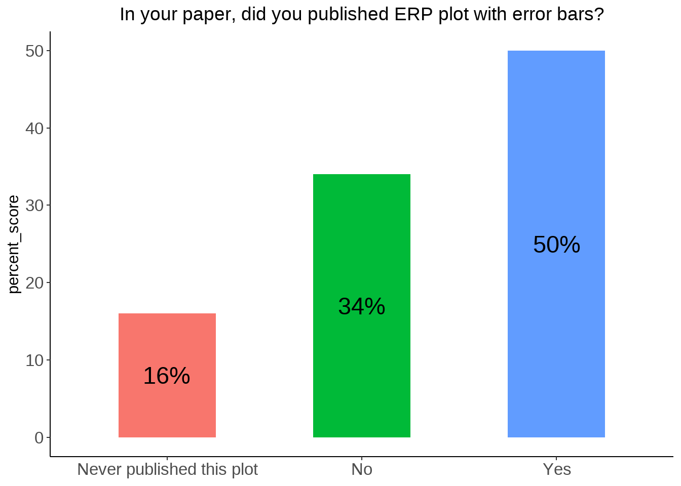

Code

eb <- table(data[74]) %>% data.frame() %>% rename_at(vars(colnames(.)), ~ c("Position", "Scores")) %>% 
  filter(Position != "Never published this plot") %>% 
  mutate(percent_score = round(Scores / sum(Scores) * 100)) 

eb_fig <- eb %>% 
    ggplot(., aes(y = Position, x = percent_score)) + 
    geom_bar(stat = "identity", width=0.5, position = "dodge", fill ="#6BAED6") + theme_classic() +
  theme(axis.text.x = element_blank(),
        axis.title.y = element_blank(),
        legend.position="none", 
        text = element_text(family = "Lato"),
        axis.text = element_text(size = 12),
        plot.title = element_text(hjust = 0.5)) +
  geom_text(aes(label = paste0(percent_score, "%"), group = Position),  #position = position_stack(vjust = 0.5), 
            hjust = -0.2) + 
  ggtitle("In your paper, have you published\nan ERP plot with error bars?")+
scale_fill_manual(values=colours)  +
    theme(legend.position="none", plot.caption = element_text(hjust=0), axis.text = element_text(size = 10)) + 
  xlim(0, 100) + labs(y = "")

eb_fig  +
    labs(caption = sprintf("N of respondents - %d",  sum(eb$Scores)))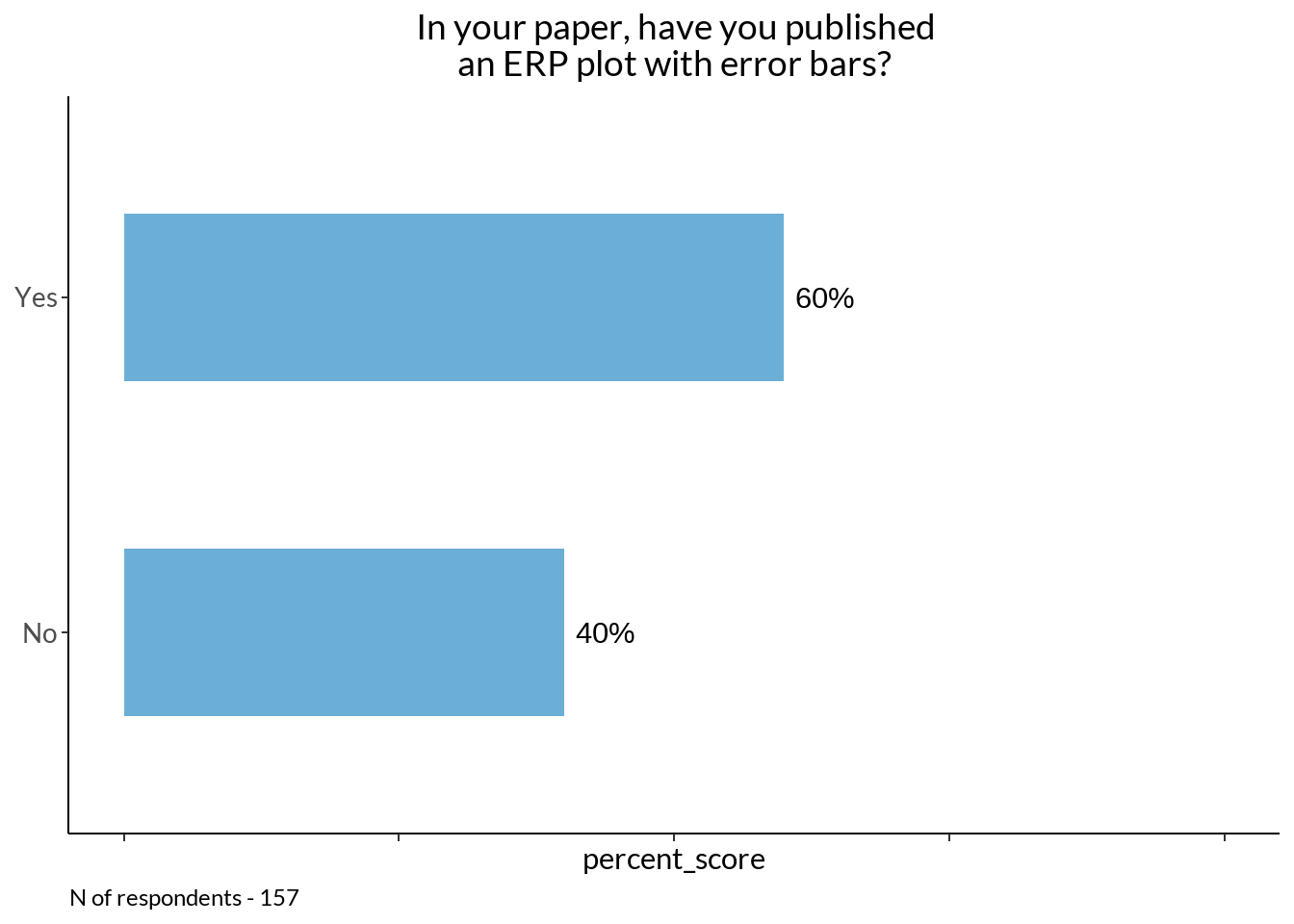

Code

ebd <- data[75] %>%  filter(!is.na(.)) %>% table()  %>% data.frame() %>% rename_at(vars(colnames(.)), ~ c("position", "scores")) %>% mutate(percent_score = round(scores / sum(scores) * 100)) %>% filter(position != "Other") 

ebd_fig <- ebd %>% 
    ggplot(., aes(y = position, x = percent_score)) + 
    geom_bar(position = "dodge", stat = "identity", width=0.5, fill ="#6BAED6") + 
    theme_classic() +
    theme(axis.text.x = element_blank(), 
          text = element_text(family = "Lato"),
          legend.position="none", 
          axis.title.y = element_blank(),
          plot.title = element_text(hjust = 0.5)) + 
     
  geom_text(aes(label = paste0(percent_score, "%"), group = position),  hjust = -0.2) + 
  ggtitle("In your figure, what\ndid the error bars represent?")+
    scale_fill_manual(values=colours) + scale_y_discrete(labels = c("Standard error\nof the mean", "Confidence\ninterval")) +
    theme(plot.caption = element_text(hjust=0), axis.text = element_text(size = 10)) + xlim(0, 100) 

ebd_fig +
    labs(caption = sprintf("N of respondents - %d",  sum(ebd$scores)))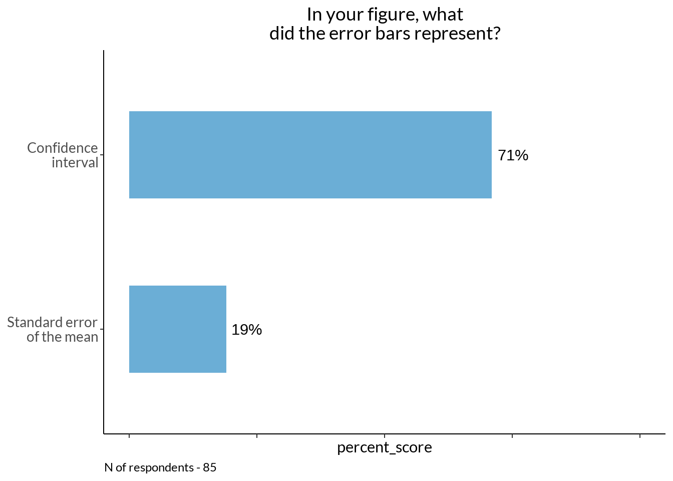 

Combined

Code

ggarrange(eb_fig + labs(x = "Percent of respondents"), ebd_fig + labs(x = "Percent of respondents"),  
          labels = c("A", "B"),
          ncol = 2, nrow = 2, align = 'h')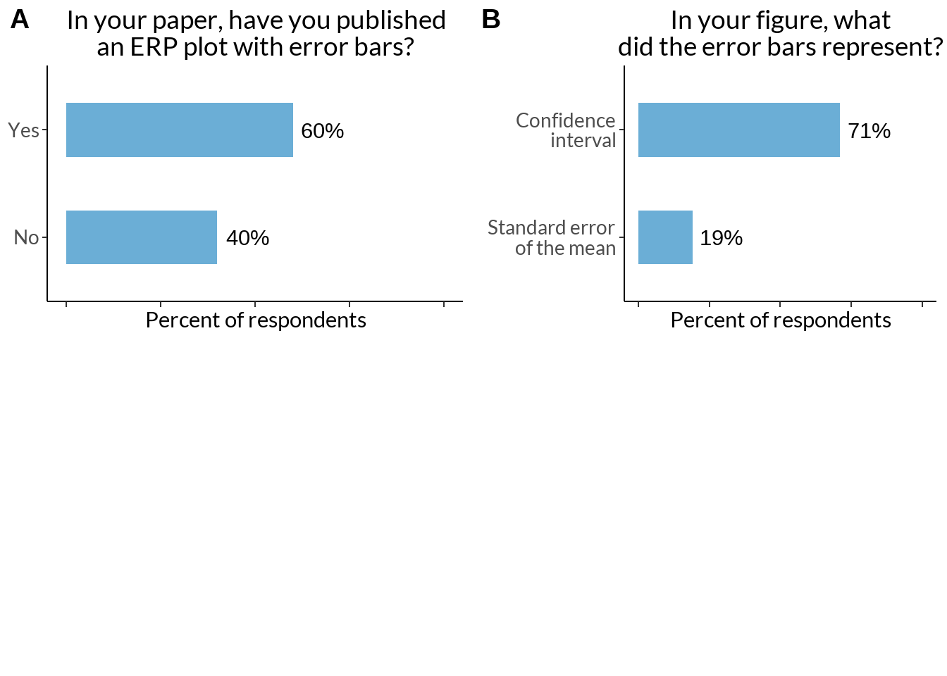  

Code

data[76] %>%  filter(!is.na(.)) %>% table()

G03Q15[other]. What did the error bars depict in your figure? [Other]
                                            - 
                                            1 
68% CI, which is close to SEM under normality 
                                            1 
                    95% ci over channel means 
                                            1 
          i'm not sure but i think it was sem 
                                            1 
                             I don't remember 
                                            1 
        median absolute deviaton or quantiles 
                                            1 
                                           NA 
                                            1 
                                           Sd 
                                            1 
 SEM, corrected for within-participant design 
                                            1 

Colormaps

Code

cb <- table(data[117]) %>% data.frame() %>% rename_at(vars(colnames(.)), ~ c("position", "scores")) 
cb  %>% 
  mutate(percent_score = round(scores / sum(scores) * 100)) %>% 
    ggplot(., aes(y = position, x = percent_score)) + #, fill = as.factor(percent_score))) +
    geom_bar(position = "dodge", stat = "identity", width=0.5, fill ="#6BAED6") + 
    theme_classic() +
    theme(
      text = element_text(family = "Lato"),
      legend.position="none", 
      strip.background = element_blank(), 
      axis.title.y = element_blank(),
      axis.text.x = element_blank(),
      axis.text.y = element_text(color = "grey10", size = 16),
      axis.title.x = element_text(color = "grey10", size = 16),
      plot.title = element_text(color = "grey10", size = 18, face = "bold", margin = margin(t = 15)),
      plot.title.position = "plot",
      plot.caption = element_text(hjust=0), 
    ) + xlab("Percent of respondents") +

  geom_text(aes(label = paste0(percent_score, "%"), group = position),  hjust = -0.2, size = 7) + 
  ggtitle("Are you aware about\nperceptual controvercies of colormaps?")+
    scale_fill_manual(values=colours) +
    theme(legend.position="none", plot.caption = element_text(hjust=0)) + xlim(0, 65) #+

Code

    labs(caption = sprintf("N of respondents - %d",  sum(cb$scores)))  

$caption
[1] "N of respondents - 213"

attr(,"class")
[1] "labels"

Colorbars

Code

rbind(table(data[117]) %>% data.frame() %>% 
  rename_at(vars(colnames(.)), ~ c("answer", "scores")) %>% 
  mutate(questions = "Awareness about\ncontrovercies of\ncolorbars")%>%
  mutate(percent_score = round(scores / sum(scores) * 100)),

table(data[118]) %>% data.frame() %>% 
  rename_at(vars(colnames(.)), ~ c("answer", "scores")) %>% 
  mutate(questions = "Awareness about\n2D colorbars") %>%
  mutate(percent_score = round(scores / sum(scores) * 100))
) %>% 
  
  ggplot(., aes(x = percent_score, y = questions, fill = answer)) +
  geom_col(stat = "identity", width = 0.5) +
   geom_text(aes(label = paste0(percent_score, "%", "\n(", answer, ")")), 
            position = position_stack(vjust = 0.5), size = 4) + 
    theme_classic()+ 
  theme(plot.title = element_text(hjust = 0.5),
        axis.text = element_text(size = 12),
        axis.title = element_text(size = 14, face = "bold"),
        legend.position = "none",
        legend.title = element_blank(),
        axis.title.y=element_blank()
        ) +
  scale_color_manual(values = c("#FF6666", "#66CC66")) +
  scale_fill_manual(values = c("#FF6666", "#66CC66"))  +
  labs(x="Percent score") +
    labs(caption = sprintf("N of respondents - %d",  sum(cb$scores))) +
    theme(legend.position="none", plot.caption.position = "plot", plot.caption = element_text(hjust=0), axis.text = element_text(size = 10))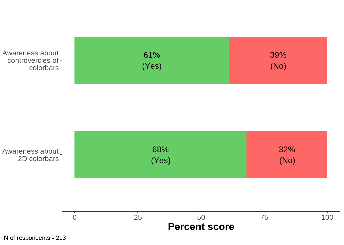 

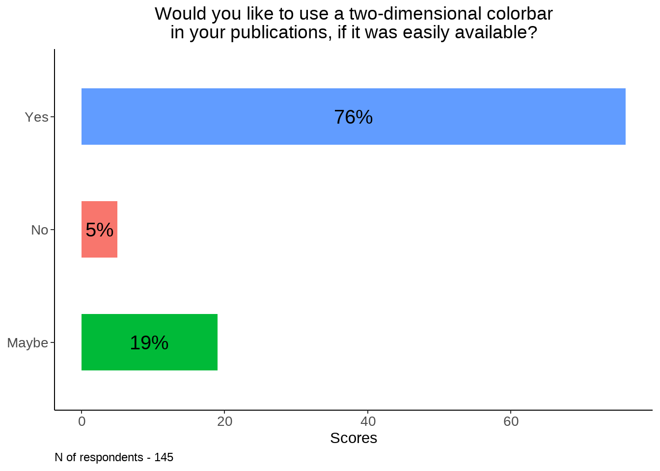
Code

tdc <- table(data[119])  %>% data.frame() %>% rename_at(vars(colnames(.)), ~ c("position", "scores")) %>%
  mutate(percent_score = round(scores / sum(scores) * 100)) 

tdc %>% 
  ggplot(., aes(y = position, x = percent_score, fill = as.factor(percent_score))) +
    geom_bar(stat = "identity", width=0.5)  + theme_classic() +
     theme(axis.title.y=element_blank(), 
        legend.position="none", 
        axis.text = element_text(size = 12),
        plot.title = element_text(hjust = 0.5)) + labs(x = "Scores") +
  geom_text(aes(label = paste0(percent_score, "%") , 
                group = position), position = position_stack(vjust = 0.5), size = 5) + 
  ggtitle("Would you like to use a two-dimensional colorbar\nin your publications, if it was easily available?") +
    labs(caption = sprintf("N of respondents - %d",  sum(tdc$scores))) +
    theme(legend.position="none", plot.caption = element_text(hjust=0), axis.text = element_text(size = 10))