Proficiency

Here we assess how proficiency in EEG affects researcher’s awareness, preferences and choices.

Setup

Code

data <- read_excel("../data/results_survey.xlsx")
data <- data[1:121] %>% 
  filter(.[[18]] !='Yes', .[[20]] < 80) # not analysed any EEG method

Proficiency factor

Code

m = FAMD(exp_data[1:5], ncp=2, axes=c(1,2))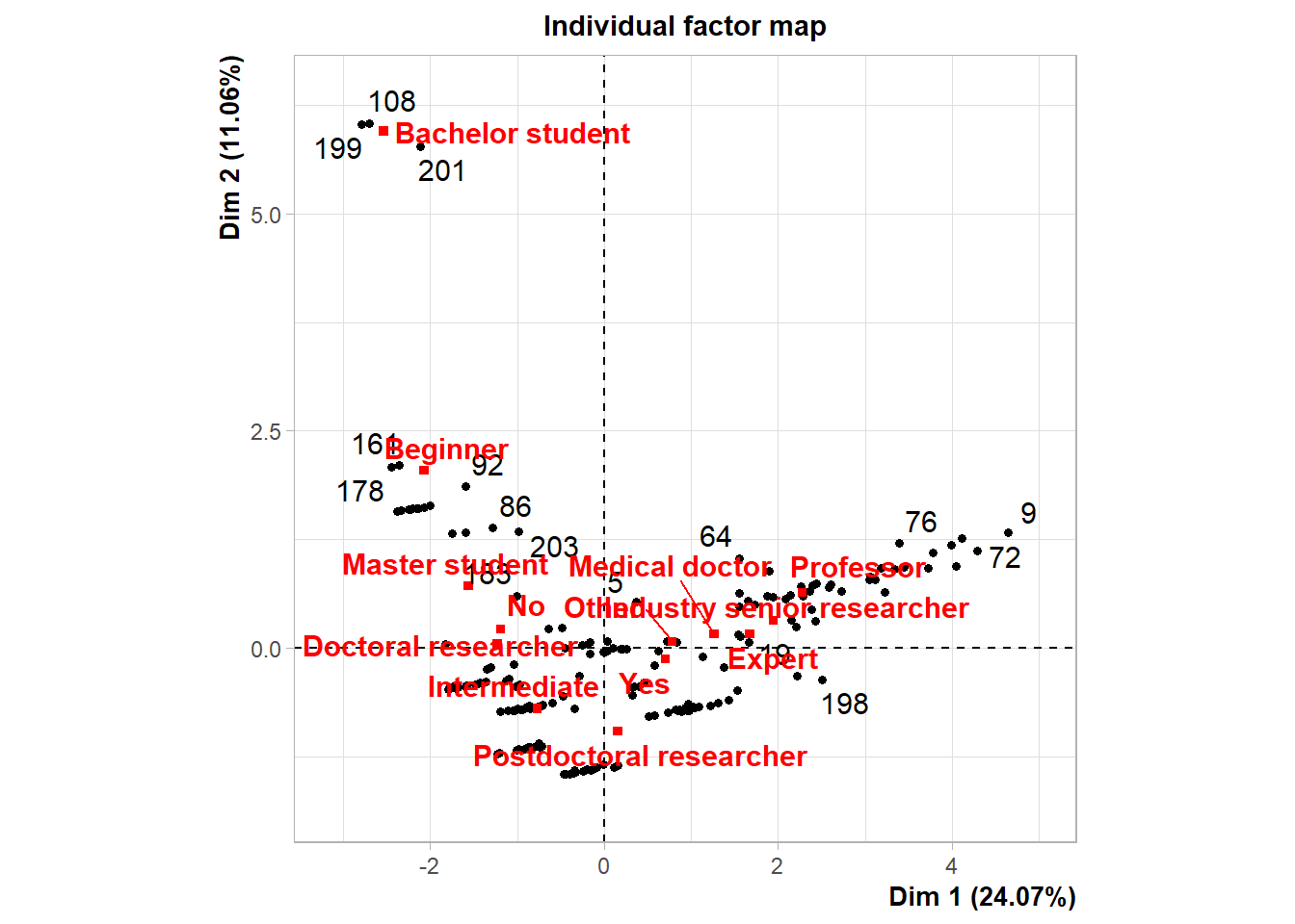

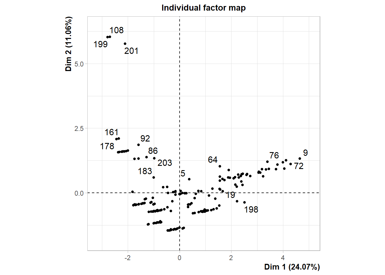
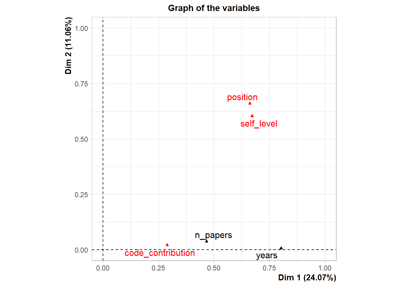
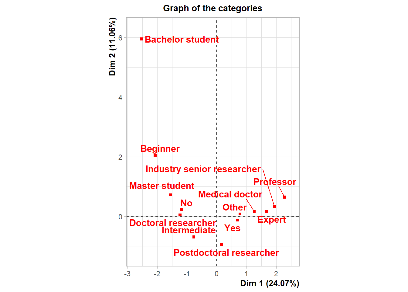
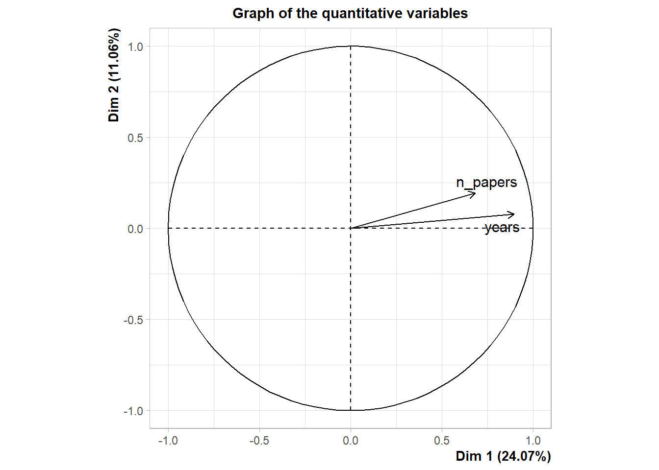
test

Proxy Proficiency should definitely correlate with years of experience

Code

factor_scores <- as.data.frame(m$ind$coord)
head(factor_scores)

       Dim.1      Dim.2
1 -1.3787967 -0.4011946
2 -1.1019372 -0.7171748
3 -0.2238351 -1.4057025
4  0.5125602 -0.7813393
5  0.3645902  0.5355694
6  1.3044242 -0.6310768

Code

cbind(data[20], factor_scores[1])  %>% 
   rename_at(vars(colnames(.)), ~ c("years", "proxy")) %>% 
  with(cor.test( proxy, years)) %>% 
  broom::tidy() %>% dplyr::select(estimate, p.value)

# A tibble: 1 × 2
  estimate  p.value
     <dbl>    <dbl>
1    0.895 5.52e-75

Tiles

controvercies

Here we cor.tests

• n_soft - number of software used
• rate - rate of electrodes recorded to electrodes analysed

Code

vec <- names(data[25:50]) %>% str_split_i(., "\\? \\[", 2) %>%  str_sub(., 1, -2)

cor_fun <- function(df){
  p.value <- cor.test(df$proxy, df$score, method = "spearman")$p.value
  mod <- spearman.ci(df$proxy, df$score) %>% tidy() %>% cbind(p.value) 
  }

n_soft <- data[25:50] %>%
  rename_at(vars(colnames(.)), ~ vec) %>% 
  mutate_at(vars(vec), function(., na.rm = FALSE) (x = ifelse(.=="Yes", 1, 0)))%>%
  rowSums() %>% tibble()

cbind(factor_scores[1], data[23]) %>% cbind(., data[24]) %>%  cbind(., n_soft) %>%
  rename_at(vars(colnames(.)), ~ c("proxy", "measure", "analyse", "n_soft")) %>%
  dplyr::filter(analyse < 500) %>% tibble() %>% 
  mutate(rate = analyse / measure) %>% 
  dplyr::select(-analyse, -measure) %>% 
  gather(type, score, rate:n_soft) %>% 
  dplyr::group_by(., type) %>% nest() %>% 
  dplyr::mutate(., model = map(data, cor_fun)) %>% unnest() %>% 
  dplyr::select(type, estimate, method, conf.low.Inf, conf.high.Sup, p.value) %>%
  dplyr::group_by(type) %>%  slice(1) %>% mutate(estimate = round(as.numeric(estimate), 3),
                                                 CI = paste0('(' , round(conf.low.Inf, 3), ', ', round(conf.high.Sup, 3), ')'),
                                                             p.value = round(as.numeric(p.value), 2)) %>% 
  mutate(p.value = cell_spec(p.value, bold = ifelse(p.value < 0.05, TRUE, FALSE))) %>% 
  mutate(type = case_when(
    type == "n_soft" ~ "Number of softwares used",
    type == "rate" ~ "Rate of electrodes recorded to analysed"
  )) %>% select(-conf.low.Inf, -conf.high.Sup) %>% 
  kable(escape = F, booktabs = T) %>% 
  kable_minimal(full_width = F,  html_font = "Source Sans Pro")

type	estimate	method	p.value	CI
Number of softwares used	0.307	Spearman's rank correlation	0	(0.165, 0.43)
Rate of electrodes recorded to analysed	0.262	Spearman's rank correlation	0	(0.124, 0.387)

attitudes

Attitudes on 8 features of ERP visualization tools Here we use cor.tests

Code

feature <- data[52:60] %>% rename_all(., ~str_split_i(colnames(data[52:60]), "\\? \\[", 2) %>% str_sub(., 1, -2) ) %>%  
  mutate_at(c(colnames(.)), 
        funs(recode(.,
        "Very important"= 2, "Important"= 1, "Neutral"= 0,
        "Low importance"= -1, "Not at all important" = -2 )))  %>% 
  cbind(., factor_scores[1]) %>%  
  rename_at(vars(colnames(.)), ~ c("subplot", "attributes", "speed", "publicable", "reproducable", "zooming", "interactive", "gui", "coding", "proxy")) 

feature %>% 
  gather(type, score, subplot:coding) %>% 
  dplyr::group_by(., type) %>% nest() %>% 
  dplyr::mutate(., model = map(data, cor_fun)) %>% unnest() %>% 
  dplyr::select(type, estimate, conf.low.Inf, conf.high.Sup, p.value) %>% # , method
  dplyr::group_by(type) %>%  slice(1) %>% mutate(estimate = round(as.numeric(estimate), 2),
                                                 CI = paste0('(' , round(conf.low.Inf, 3), ', ', round(conf.high.Sup, 3), ')' ),
                                                             p.value = round(as.numeric(p.value), 2)) %>% 
  mutate(p.value = cell_spec(p.value, bold = ifelse(p.value < 0.05, TRUE, FALSE))) %>% 
  dplyr::rename(`Software feature` = type, `Spearman rho` = estimate) %>% 
  select(-conf.low.Inf, -conf.high.Sup) %>% 
  kable(escape = F, booktabs = T) %>% 
  kable_minimal(full_width = F,  html_font = "Source Sans Pro") 

Software feature	Spearman rho	p.value	CI
attributes	-0.07	0.32	(-0.223, 0.074)
coding	0.17	0.01	(0.03, 0.301)
gui	-0.13	0.07	(-0.264, 0.018)
interactive	-0.07	0.34	(-0.209, 0.06)
publicable	-0.11	0.11	(-0.243, 0.025)
reproducable	0.07	0.33	(-0.072, 0.199)
speed	0.02	0.82	(-0.121, 0.151)
subplot	0.12	0.08	(-0.024, 0.248)
zooming	-0.01	0.92	(-0.141, 0.122)

awareness

Code

log_fun <- function(df){
  mod <- glm(df$score ~ df$proxy, family = "binomial") 
  ci1 <- confint(mod)[2]
  ci2 <- confint(mod)[4]
  mod %>% tidy() %>% slice(-1) %>% cbind(ci1) %>% cbind(ci2)
}

Code

cbind(factor_scores[1], data[79]) %>% cbind(., data[117]) %>% 
  cbind(., data[118]) %>% 
  rename_at(vars(colnames(.)), ~ c("proxy", "ud", "jet_aware", "twod_aware")) %>%
  mutate(ud = ifelse(ud=="Up", 1, 0), 
         jet_aware = ifelse(jet_aware =="Yes", 1, 0),
         twod_aware = ifelse(twod_aware =="Yes", 1, 0)) %>% 
  gather(type, score, ud:twod_aware) %>% 
  dplyr::group_by(., type) %>% nest() %>% 
  dplyr::mutate(., model = map(data, log_fun)) %>% unnest() %>% 
  dplyr::select(type, estimate, std.error, p.value, ci1, ci2) %>%
  dplyr::group_by(type) %>%  slice(1) %>% mutate(p.value = round(as.numeric(p.value), 3),
                                                 estimate = round(as.numeric(estimate), 3),
                                                 std.error = round(as.numeric(std.error), 3),
                                                CI = paste0('(' , round(ci1, 3), ', ', round(ci2, 2), ')' )) %>%
  dplyr::select(-ci1, -ci2) %>%
  mutate(p.value = cell_spec(p.value, bold = ifelse(p.value < 0.05, TRUE, FALSE))) %>% 
  mutate(type = case_when(
    type == "ud" ~ "Polaritiy convention: up",
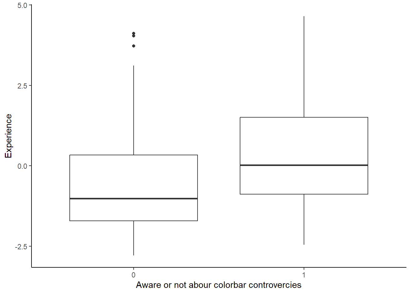
    type == "jet_aware" ~ "Awareness about colorbar perceptual controvercies: yes",
    type == "twod_aware" ~ "Awareness about 2D colobars: yes"
  )) %>% 
  dplyr::rename(`Visualisation customs` = type) %>% 
  kable(escape = F, booktabs = T) %>% 
  kable_minimal(full_width = F,  html_font = "Source Sans Pro")

Visualisation customs	estimate	std.error	p.value	CI
Awareness about colorbar perceptual controvercies: yes	0.335	0.095	0	(0.156, 0.53)
Awareness about 2D colobars: yes	0.112	0.090	0.213	(-0.061, 0.29)
Polaritiy convention: up	-0.022	0.111	0.843	(-0.236, 0.2)

tools

Code

vec <- names(data[25:51]) %>% str_split_i(., "\\? \\[", 2) %>%  str_sub(., 1, -2)

data[25:51] %>%
  rename_at(vars(colnames(.)), ~ vec) %>% 
  dplyr::select(-Other) %>% 
  mutate_at(vars(vec[1:26]), function(., na.rm = FALSE) (x = ifelse(.=="Yes", 1, 0))) %>%
  select_if(colSums(.) > 10) %>% 
  cbind(factor_scores[1], .) %>% dplyr::rename(proxy = !!names(.)[1]) %>% 
  gather(type, score, BESA:`Custom scripts`) %>% 
   dplyr::group_by(., type) %>% nest() %>% 
  dplyr::mutate(., model = map(data, log_fun)) %>% unnest() %>% 
  dplyr::select(type, estimate, std.error, p.value, ci1, ci2) %>%
  dplyr::group_by(type) %>%  slice(1) %>% mutate(p.value = round(as.numeric(p.value), 2), 
                                                 estimate = round(as.numeric(estimate), 2),
                                                 std.error = round(as.numeric(std.error), 2), 
                                                 CI = paste0('(' , round(ci1, 3), ', ', round(ci2, 3), ')' )) %>%
  dplyr::select(-ci1, -ci2) %>%
  mutate(p.value = cell_spec(p.value, bold = ifelse(p.value < 0.05, TRUE, FALSE))) %>% 
  dplyr::rename(`Analytical software` = type) %>% 
  kable(escape = F, booktabs = T) %>% 
  kable_minimal(full_width = F,  html_font = "Source Sans Pro")

Analytical software	estimate	std.error	p.value	CI
BESA	0.18	0.16	0.26	(-0.143, 0.482)
Brain Vision Analyser	0.02	0.10	0.81	(-0.172, 0.212)
Brainstorm	0.15	0.10	0.16	(-0.063, 0.35)
Custom scripts	0.13	0.08	0.13	(-0.036, 0.294)
EEGLAB	0.25	0.09	0.01	(0.079, 0.443)
ERPLAB	0.19	0.10	0.04	(0.006, 0.384)
FieldTrip	0.19	0.08	0.02	(0.028, 0.357)
LIMO	0.34	0.15	0.02	(0.049, 0.627)
MNE-Python	-0.05	0.08	0.52	(-0.219, 0.108)
SPM	0.09	0.14	0.53	(-0.197, 0.356)
Unfold	0.08	0.16	0.61	(-0.254, 0.391)

Proficiency and …

Tools

Code

cbind(factor_scores[1], data[31]) %>% 
  rename_at(vars(colnames(.)), ~ c("proxy", "EEGLAB")) %>%
  mutate(EEGLAB = ifelse(EEGLAB =="Yes", 1, 0)) %>% 
  ggplot(., aes(x=as.factor(EEGLAB), y = proxy)) + 
  geom_boxplot() + labs(x = "EEGLAB", y = "Experience") +  
  theme_classic()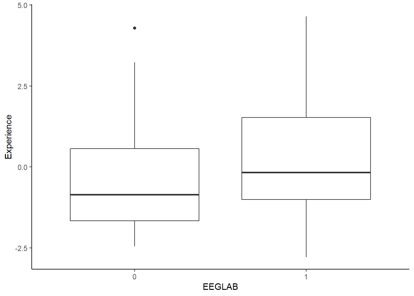

Code

cbind(factor_scores[1], data[35]) %>% 
  rename_at(vars(colnames(.)), ~ c("proxy", "ERPLAB")) %>%
  mutate(ERPLAB = ifelse(ERPLAB =="Yes", 1, 0)) %>% 
  ggplot(., aes(x=as.factor(ERPLAB), y = proxy)) + 
  geom_boxplot() + labs(x = "ERPLAB", y = "Experience") +  
  theme_classic()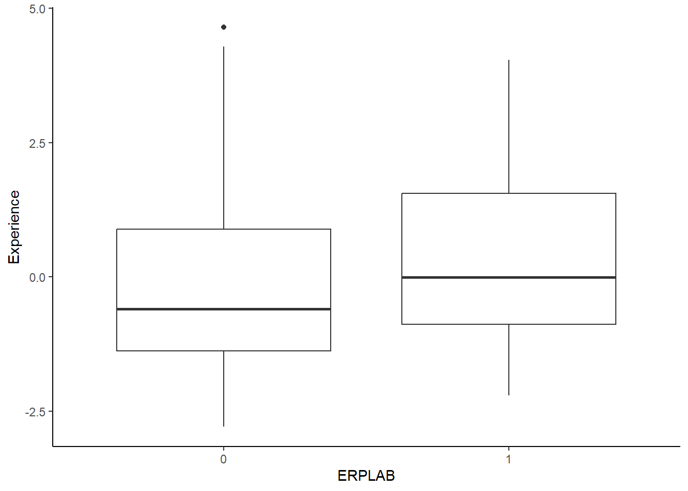

Code

cbind(factor_scores[1], data[41]) %>% 
  rename_at(vars(colnames(.)), ~ c("proxy", "Fieldtrip")) %>%
  mutate(Fieldtrip = ifelse(Fieldtrip =="Yes", 1, 0)) %>% 
  ggplot(., aes(x=as.factor(Fieldtrip), y = proxy)) + 
  geom_boxplot() + labs(x = "Fieldtrip", y = "Experience") +  
  theme_classic()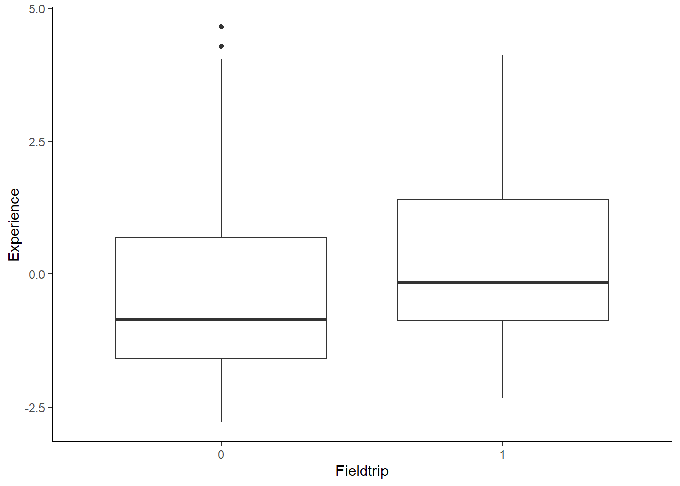

Code

cbind(factor_scores[1], data[43]) %>% 
  rename_at(vars(colnames(.)), ~ c("proxy", "LIMO")) %>%
  mutate(LIMO = ifelse(LIMO =="Yes", 1, 0)) %>% 
  ggplot(., aes(x=as.factor(LIMO), y = proxy)) + 
  geom_boxplot() + labs(x = "LIMO", y = "Experience") +  
  theme_classic()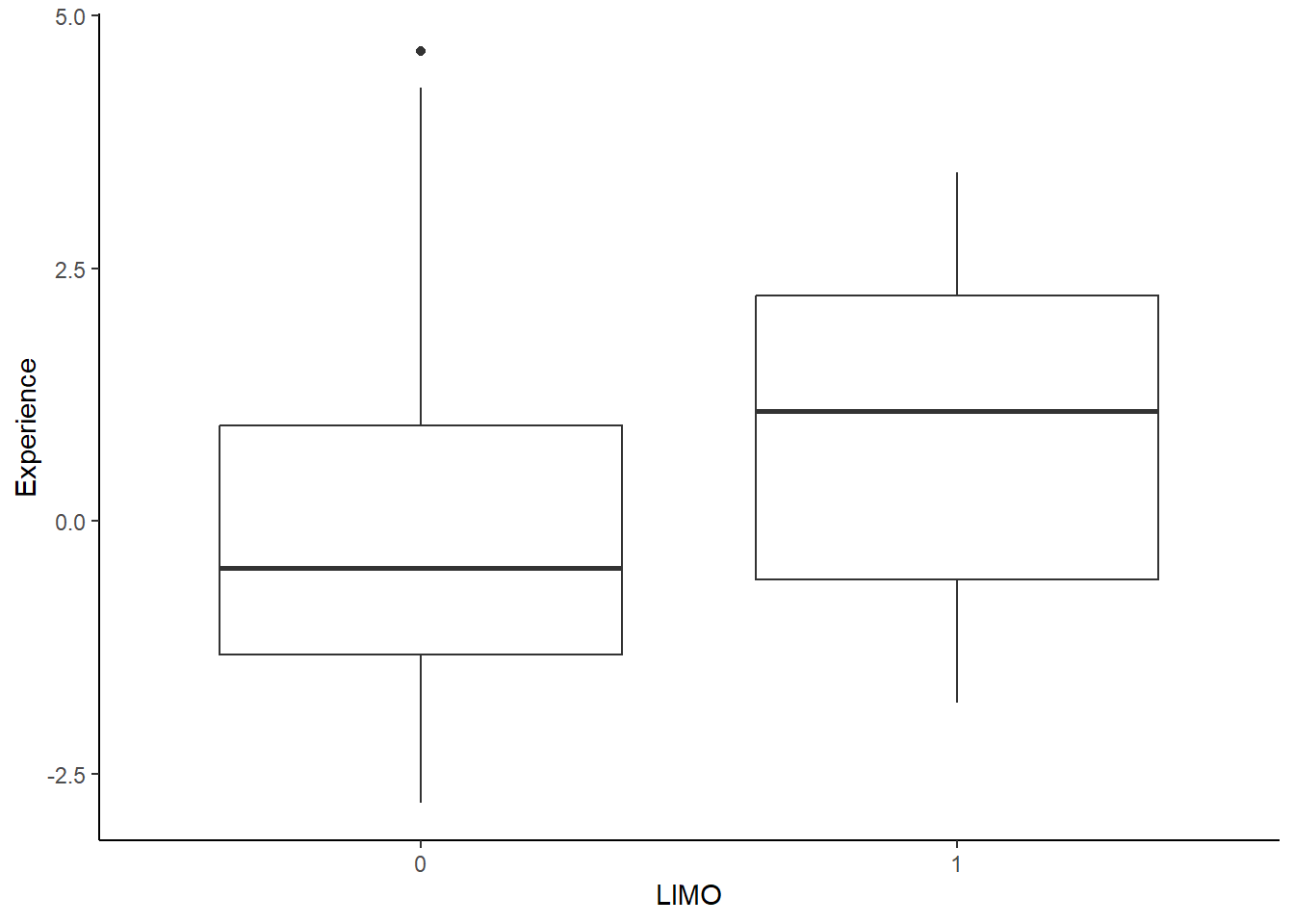

Number of used software

Code

vec <- names(data[25:50]) %>% str_split_i(., "\\? \\[", 2) %>%  str_sub(., 1, -2)

software <- data[25:50] %>%
    rename_at(vars(colnames(.)), ~ vec) %>% 
  mutate_at(vars(vec), function(., na.rm = FALSE) (x = ifelse(.=="Yes", 1, 0))) %>% rowSums() %>% tibble()

Code

cbind(data.frame(rowSums(software)), factor_scores[1])  %>% 
   rename_at(vars(colnames(.)), ~ c("n_soft", "experience")) %>% 
  filter(n_soft > 0) %>% 
  ggplot(., aes(x=n_soft, y=experience)) + geom_jitter() + geom_smooth()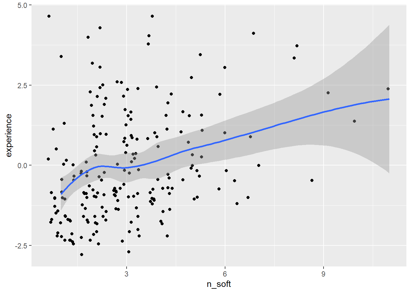

Code

cbind(data.frame(rowSums(software)), factor_scores[1])  %>% 
   rename_at(vars(colnames(.)), ~ c("n_soft", "experience")) %>% 
  filter(n_soft > 0) %>% 
  lm(data=., n_soft ~ experience) %>% summary(.)

Call:
lm(formula = n_soft ~ experience, data = .)

Residuals:
    Min      1Q  Median      3Q     Max 
-3.6473 -1.2372 -0.3383  0.9372  7.1416 

Coefficients:
            Estimate Std. Error t value Pr(>|t|)    
(Intercept)  3.02985    0.11864  25.539  < 2e-16 ***
experience   0.34813    0.07065   4.927 1.71e-06 ***
---
Signif. codes:  0 '***' 0.001 '**' 0.01 '*' 0.05 '.' 0.1 ' ' 1

Residual standard error: 1.711 on 206 degrees of freedom
Multiple R-squared:  0.1054,    Adjusted R-squared:  0.1011 
F-statistic: 24.28 on 1 and 206 DF,  p-value: 1.709e-06

Channels

Code

data %>% select(23, 24) %>% 
  cbind(., factor_scores[1]) %>% 
  rename_at(vars(colnames(.)), ~ c("measure", "analyse", "experience")) %>% 
  filter(analyse < 500) %>% 
  mutate(rate = analyse / measure) %>% 
  ggplot(., aes(x=rate, y=experience)) + 
  geom_point() +                                      
  stat_smooth(method = "lm",
              formula = y ~ x,
              geom = "smooth") +
  labs(x ="analyse / measure") +
  theme_classic()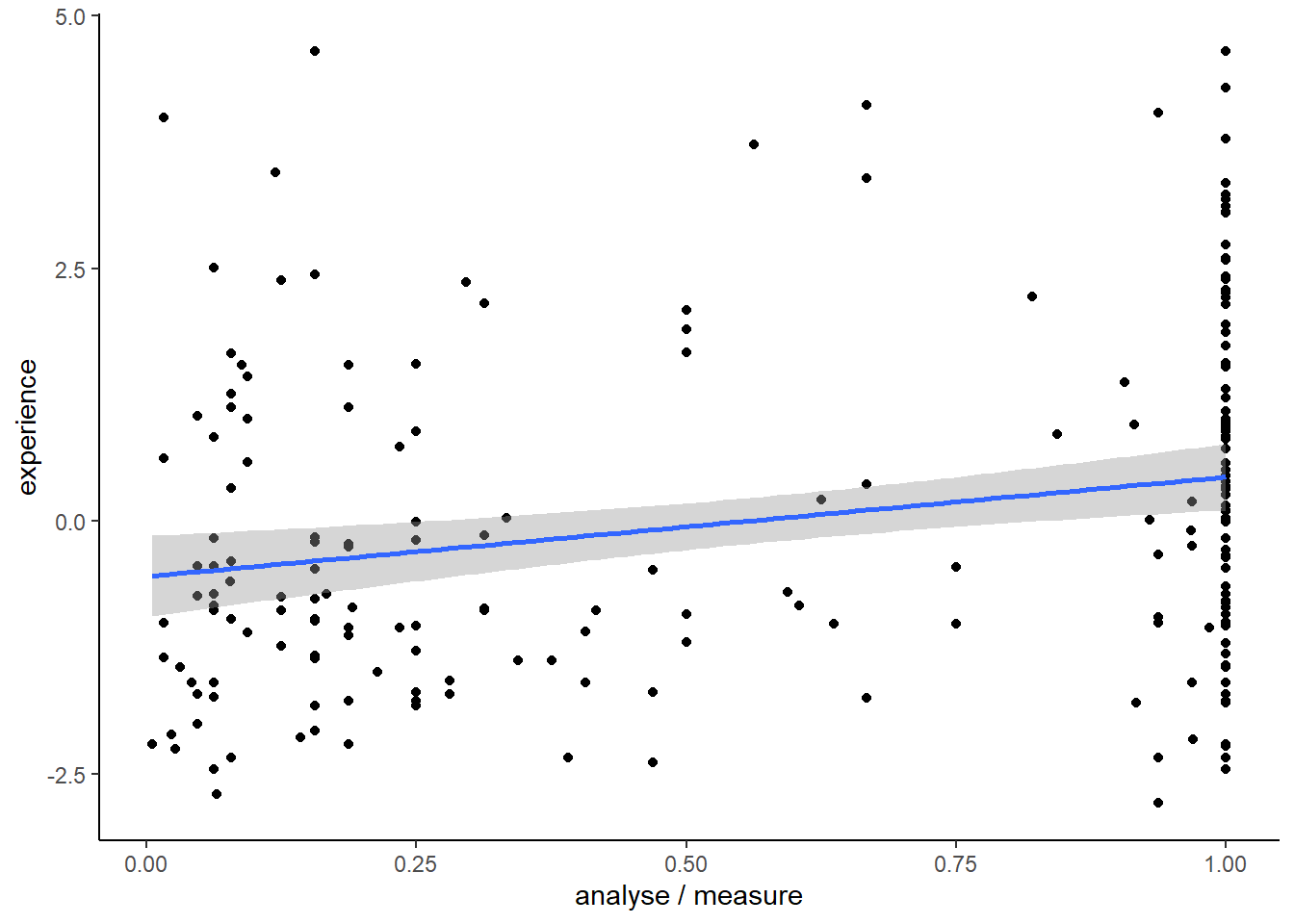

Code

data %>% select(23, 24) %>% 
  cbind(., factor_scores[1]) %>% 
  rename_at(vars(colnames(.)), ~ c("measure", "analyse", "experience")) %>% 
  filter(analyse < 500) %>% 
  mutate(rate = analyse / measure) %>%
  lm(rate ~ experience, .) %>% summary()

Call:
lm(formula = rate ~ experience, data = .)

Residuals:
    Min      1Q  Median      3Q     Max 
-0.7854 -0.3809  0.0336  0.3843  0.5565 

Coefficients:
            Estimate Std. Error t value Pr(>|t|)    
(Intercept)  0.57967    0.02740  21.156  < 2e-16 ***
experience   0.05554    0.01615   3.439 0.000708 ***
---
Signif. codes:  0 '***' 0.001 '**' 0.01 '*' 0.05 '.' 0.1 ' ' 1

Residual standard error: 0.3942 on 205 degrees of freedom
Multiple R-squared:  0.05454,   Adjusted R-squared:  0.04992 
F-statistic: 11.82 on 1 and 205 DF,  p-value: 0.0007079

n_plot

Code

n_soft <- data[25:50] %>%
    rename_at(vars(colnames(.)), ~ vec) %>% 
  mutate_at(vars(vec), function(., na.rm = FALSE) (x = ifelse(.=="Yes", 1, 0))) %>% rowSums() %>% tibble()

cbind(n_soft, factor_scores[1]) %>% 
  rename_at(vars(colnames(.)), ~ c("n_soft", "experience")) %>% 
  ggplot(., aes(x=n_soft, y=experience)) + 
  geom_point() +                                      
  stat_smooth(method = "lm",
              formula = y ~ x,
              geom = "smooth") +
  labs(x ="n_soft") +
  theme_classic()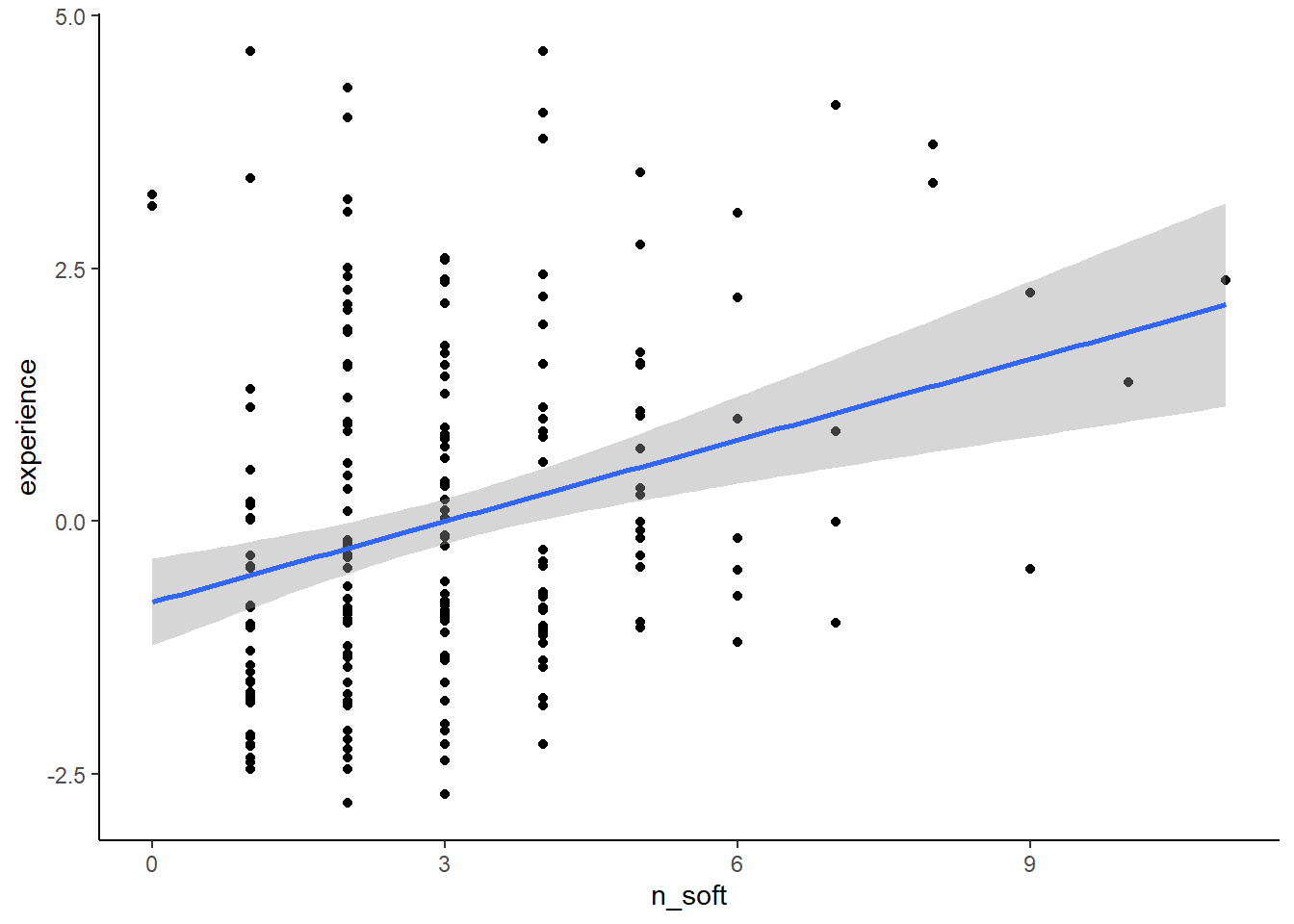

jet awareness

Code

cbind(factor_scores[1], data[117]) %>% 
  rename_at(vars(colnames(.)), ~ c("proxy", "jet_aware")) %>%
  mutate(jet_aware = ifelse(jet_aware =="Yes", 1, 0)) %>% 
  ggplot(., aes(x=as.factor(jet_aware), y = proxy)) + 
  geom_boxplot() + labs(x = "Aware or not abour colorbar controvercies", y = "Experience") +  
  theme_classic()