All figures

Here are the figures from the paper Art of the Brainwaves.

data

Code

data <- read_excel("../data/results_survey.xlsx")
data <- data[1:121] %>% 
  filter(.[[18]] !='Yes') # not analysed any EEG method

cit1 <- read.table(file = "../data/cit/eeglab.txt", header = TRUE, fill = TRUE)[1:2] %>% mutate(name = "EEGLAB")
cit2 <- read.table(file = "../data/cit/mne.txt", header = TRUE, fill = TRUE)[1:2]%>% mutate(name = "MNE")
cit3 <- read.table(file = "../data/cit/erplab.txt", header = TRUE, fill = TRUE)[1:2]%>% mutate(name = "ERPLAB")
cit4 <- read.table(file = "../data/cit/fieldtrip.txt", header = TRUE, fill = TRUE)[1:2]%>% mutate(name = "FieldTrip")
cit5 <- read.table(file = "../data/cit/brainstorm.txt", header = TRUE, fill = TRUE)[1:2]%>% mutate(name = "Brainstorm")

cit_data <- rbind(cit1, cit2, cit3, cit4, cit5) %>% rename_at(vars(colnames(.)), ~ c("year", "citations", "name"))

just <- read.csv("../data/justification.csv") %>% dplyr::select(group, num)

font_add_google("Lato")
showtext_opts(dpi = 200)
showtext_auto(enable = TRUE)

Figure 4

Code

country <- data.frame(table(data[8]))  %>% dplyr::rename(country_work = !!names(.)[1]) %>%
  mutate(country_work = ifelse(Freq >= 6, as.character(country_work), "Other")) %>% group_by(country_work) %>% 
  mutate(country_work = case_when(
    country_work == "United Kingdom" ~ "UK",
    TRUE ~ as.character(country_work)  
  )) %>% 
  dplyr::summarise(Freq = sum(Freq)) %>% 
  dplyr::mutate(percent_score = round(Freq / sum(Freq) * 100)) %>% 
  mutate(country_work = factor(country_work, levels = country_work[rev(order(percent_score))]))

italised1 <- rev(c("Germany", expression(italic("Other")), "USA", "UK", "France", "Netherlands", "Switzerland", "Spain", "Italy", "Russia", "Belgium", "Australia"))


country_fig <- country %>%
  ggplot(data = ., aes(y = reorder(country_work, percent_score),  x= percent_score)) +#, fill = country_work)) +
  geom_col(stat = "identity", width = 0.8) + 
  labs(x = "Percent", y="", title = "Country of work") +
  geom_text(aes(label = paste0(percent_score, "%")), hjust = -0.1,
  size = 4)  + theme_classic()   +
  theme(legend.position="none", 
        plot.caption.position = "plot", 
        plot.caption = element_text(hjust=0), 
        axis.text.y = element_text(size = 12),
        text = element_text(family = "Lato"),
        ) + coord_cartesian(clip = "off") +
    scale_y_discrete(labels = italised1)


pos <- data[c(12, 13)] %>% dplyr::rename(position = !!names(.)[1], other = !!names(.)[2]) %>%
  mutate(position = case_when(
    position == "Industry senior researcher" ~ "Industry R&D",
    position == "Doctoral researcher" ~ "PhD Candidate",
    position == "Postdoctoral researcher" ~ "Postdoc",
    position == "Bachelor student" ~ "Bachelor",
    position == "Master student" ~ "Master",
    TRUE ~ as.character(position)))  %>% 
  mutate(other = tolower(other)) %>% 
  mutate(position = case_when(
      grepl("\\b(master)\\b", other) == TRUE ~ "Master",
      grepl("\\b(engineer|tech)\\b", other) == TRUE ~ "Industry R&D",
      TRUE ~ as.character(position)
      )) %>% dplyr::select(position) %>% na.omit(.) %>% table() %>% as.data.frame()  %>% 
   mutate(position = factor(position, levels = rev(c('Bachelor', 'Master', 'PhD Candidate', 'Postdoc', 'Professor', 'Industry R&D', 'Medical doctor', 'Other')))) %>% mutate(percent_score = round(Freq / sum(Freq) * 100))

italised2 <- rev(c('Bachelor', 'Master', 'PhD Candidate', 'Postdoc', 'Professor', 'Industry R&D', 'Medical doctor', expression(italic('Other'))))
position <- pos %>% 
    ggplot(data = ., aes(y = position, x= percent_score))+ 
    geom_col(stat="identity") + labs(title = "Current position", x = "Percent", y="") +
    geom_text(aes(label = paste0(percent_score, "%")), hjust = -0.1) +
    theme_classic()  +
    theme(legend.position="none", 
        text = element_text(family = "Lato"), 
        plot.caption.position = "plot", 
        plot.caption = element_text(hjust=0), 
        axis.text = element_text(size = 10)) + 
    coord_cartesian(clip = "off") +
    scale_y_discrete(labels = italised2)

field <- as.data.frame(table(data[9])) %>% arrange(desc(Freq)) %>% head(3)
field$Freq[1] <- field$Freq[1] + 1 # from Others
field$Freq[2] <- field$Freq[2] + 1
field$Freq[3] <- field$Freq[3] + 1

fieldplot <- field %>% dplyr::rename(area = !!names(.)[1]) %>%
  mutate(percent_score = round(Freq / sum(Freq) * 100)) %>% 
    ggplot(data = ., aes(y = reorder(area, percent_score),  x = percent_score)) +
    geom_col(stat="identity", width = 0.7) + labs(y = "", title="Field of research", x ="Percent") +
    geom_text(aes(label = paste0(percent_score, "%")), hjust = -0.1)  + 
  theme_classic()  +
    theme(legend.position="none", 
          plot.caption = element_text(hjust=0), 
          text = element_text(family = "Lato"),
          axis.text.y = element_text(size = 12)) + scale_y_discrete(labels=c("Applied", "Clinical", "Fundamental")) + 
  coord_cartesian(clip = "off")

method <- data[14:17]
colnames(method) <- names(method) %>%  str_split_i(., "\\? \\[", 2)  %>%  str_sub(., 1, -2)

methods <- data.frame(rowSums(t(data.frame(foreach(i = colnames(method)) %do% ifelse(method[i]=="Yes", 1, 0))))) %>% 
  tibble::rownames_to_column(., "plots") %>% 
    dplyr::rename(method = !!names(.)[1], sum_scores = !!names(.)[2])  %>%  
    mutate(percent_score = round(sum_scores / sum(sum_scores) * 100)) %>% 
  
    ggplot(., aes(y = reorder(method, percent_score), x = percent_score)) + 
    geom_col(stat = "identity", width = 0.7) + labs(y = "", x = "Percent", title = "Method") +
    geom_text(aes(label = paste0(percent_score, "%")), hjust = -0.1)+
    theme_classic() + 
    theme(legend.position="none", text = element_text(family = "Lato"), 
          plot.caption = element_text(hjust=0), axis.text.y = element_text(size = 14)) +
    scale_y_discrete(labels=c("OPMs MEG", "Intracranial EEG", "SQUID MEG", "Scalp EEG")) +
    coord_cartesian(clip = "off") + xlim(0, 75)

Code

f4 <- ggarrange(country_fig + geom_col(stat = "identity", width = 0.8, fill ="#6BAED6") + 
            theme(axis.text.y = element_text(size = 12), plot.title = element_text(size = 14), axis.text.x = element_blank()) + xlim(0, 100) + labs(x= "Percentage of respondents"), 
          position + xlim(0, 100) + geom_col(stat = "identity", fill ="#6BAED6") + 
            theme(axis.text.y = element_text(size = 12), plot.title = element_text(size = 14), axis.text.x = element_blank()) + labs(x = "Percentage of respondents"),   
          fieldplot + xlim(0, 100) + geom_col(stat = "identity", width = 0.7, fill ="#6BAED6") + 
            theme(axis.text.y = element_text(size = 12), plot.title = element_text(size = 14), axis.text.x = element_blank()) + labs(x = "Percentage of respondents"), 
          methods  + geom_col(stat = "identity", width = 0.7, fill ="#6BAED6") +  
            scale_y_discrete(labels=c("OPMs", "iEEG", "MEG", "Scalp EEG")) + xlim(0, 100) +  
            theme(axis.text.y = element_text(size = 12), plot.title = element_text(size = 14), axis.text.x = element_blank()) + labs(x = "Percentage of respondents"),
          labels = c("A", "B", "C", "D"),
          ncol = 2, nrow = 2, align = 'hv') 

f4 

Code

ggsave("../figures_jpg/Figure 4.jpg", f4, units = "px", dpi=100, width = 1500, height = 938)
ggsave("../figures_png/Figure 4.png", f4, units = "px", dpi=100, width = 1500, height = 938)

Figure 5

Code

year <- data %>% dplyr::rename(years = !!names(.)[20]) %>% filter(.[[20]] < 50) %>% select(years)

years <- year %>% group_by(years) %>% 
  dplyr::summarise(n = n()) %>% 
  mutate(p = round(n / sum(n), 2))  %>% ggplot(data = ., aes(x=years, y = p)) +
  geom_col(position = "identity", col="grey") +  scale_x_continuous(breaks=seq(0, 30, 5)) +
  labs(title ="Years of experience", y= "Percentage of\nrespondents", x="")  +
  theme_classic() + theme(legend.position="none", text = element_text(family = "Lato"),
                          axis.text = element_text(size = 10)) +
  theme(legend.position="none", plot.caption = element_text(hjust=0), 
        axis.text = element_text(size = 10)) + 
  geom_vline(xintercept = median(year$years),        # Add line for mean
             col = "brown1", lty='dashed',
             lwd = 1) +
  geom_text(aes(label = paste0("median = ", median(year$years)), col = "brown1",
                x = median(year$years)*2.2, family = "Lato",
                y  = 0.11)) + scale_y_continuous(labels = scales::percent)
tmp_med <- data[19] %>% dplyr::rename(papers = !!names(.)[1]) %>% 
  filter(papers < 100) %>% summarise(median_paper = median(papers)) %>% as.numeric()

papers <- data[19] %>% dplyr::rename(papers = !!names(.)[1]) 

papers_fig <- papers %>% 
  filter(papers < 100) %>% group_by(papers) %>% 
  dplyr::summarise(n = n()) %>% 
  mutate(p = round(n / sum(n), 2)) %>% 

ggplot(., aes(x = papers, y = p)) +
  geom_col(position = "identity", bins = 45, col="grey") +
  labs(x ="The number of published papers/preprints with EEG, MEG or iEEG analysis", y = "") + theme_classic()  +
  theme(legend.position="none", plot.caption = element_text(hjust=0), text = element_text(family = "Lato"),
        axis.text = element_text(size = 10)) + 
  geom_vline(xintercept = tmp_med - 1,        # Add line for mean, -1 because starts from zero
             col = "brown1", lty='dashed',
             lwd = 1) +
  geom_text(aes(label = paste0("median = ", tmp_med), 
                x = tmp_med*7, col = "brown1", family = "Lato",
                y  = 0.15)) + scale_y_continuous(labels = scales::percent)

cc <- table(data[22])  %>% data.frame()%>% dplyr::rename(level = !!names(.)[1]) %>%
    mutate(percent_score = round(Freq / sum(Freq) * 100)) %>% 
    ggplot(data = ., aes(y = reorder(level, Freq),  x = percent_score))  +
    geom_col(stat="identity", width = 0.5) + 
    geom_text(aes(label = paste0(percent_score, "%")), hjust = -0.2)  +
  theme_classic() +
  theme(legend.position="none", axis.text.x = element_text(size = 12), text = element_text(family = "Lato")) +
  labs(title = "Code contribution", x="Percentage", y="")  +
    theme(legend.position="none", plot.caption = element_text(hjust=0), axis.text = element_text(size = 10)) + xlim(0, 64)

colorsal <- c("#f9a65a", "#599ad3", "#8dc63f")
sal <- table(data[21]) %>% data.frame() %>% dplyr::rename(level = !!names(.)[1]) %>%
    mutate(percent_score = round(Freq / sum(Freq) * 100)) %>% 
    mutate(level = factor(level, levels = rev(c("Beginner", "Intermediate", "Expert"))))

sall <- sal %>% 
    ggplot(data = ., aes(y = level, x = percent_score)) +  
    geom_col(stat="identity",  width = 0.5) + labs(x = "Percentage", y = "", title="Self-assessed level") +
    geom_text(aes(label = paste0(percent_score, "%")), hjust = -0.2)  + theme_classic() +
    theme(legend.position="none", axis.text.x = element_text(size = 12), text = element_text(family = "Lato"),
          plot.caption = element_text(hjust=0), axis.text = element_text(size = 10))

Code

f5 <- ggarrange(years +  geom_col(position = "identity", bins = 45, fill ="#6BAED6") + 
  geom_vline(xintercept = median(year$years),        # Add line for mean
             col = "#FC9272", lty='dashed',
             lwd = 1),
  
          papers_fig + geom_col(position = "identity", bins = 45, fill ="#6BAED6") + 
  geom_vline(xintercept = tmp_med - 1,        # Add line for mean
             col = "#FC9272", lty='dashed',
             lwd = 1) + labs(title ="Number of papers published", y= "Percentage of\nrespondents", x=""), 
  
          cc +  geom_col(stat = "identity",  width = 0.5, fill ="#6BAED6") + xlim(0, 100) + theme(axis.text.y = element_text(size = 10), axis.text.x = element_blank()) +  
    labs(x ="Percentage of respondents") , 
  
          sall + geom_col(stat = "identity",  width = 0.5, fill ="#6BAED6") + xlim(0, 100) + theme(axis.text.y = element_text(size = 10), axis.text.x = element_blank()) +  
    labs(x ="Percentage of respondents"), 
          labels = c("A", "B", "C", "D"),
          ncol = 2, nrow = 2) 
f5

Code

ggsave("../figures_jpg/Figure 5.jpg", f5, units = "px", dpi=150, width = 1500, height = 931)
ggsave("../figures_png/Figure 5.png", f5, units = "px", dpi=150, width = 1500, height = 931)

Figure 6

Code

vec <- c("line", "butterfly", "topo",  "topo_map", "topo_array", "erp_image", "parallel", "channel_image")

familiar <-  data[61:68] %>% rename_at(vars(colnames(.)), ~ vec) %>% 
  mutate_at(vars(vec), function(., na.rm = FALSE) (x = ifelse(.=="Yes", 1, 0)))

stat_preproc <- function(vec){
  tmp <- vec %>% filter(!is.na(.)) %>% 
    dplyr::rename(words = !!names(.)[1]) %>% mutate(words = tolower(words)) %>% 
    mutate(words = ifelse(nchar(words) < 3, paste(words, "baddd"), words)) %>% 
    mutate(check = 
    ifelse(grepl("\\b(baddd|idea|sure|confus|aware|do not|know|why|good|remember|unsure|confusing|mess|unclear|ugly|don't|useless|nan|clear)\\b", words), "bad", "good")) 
  return(tmp)
}

Code

vec_named <- names(data[ , grepl( "How would you " , names(data))])
plot_names <- c("line", "butterfly", "topo", "topo_series", "erp_grid", "erp_img", "parallel", "channel_img")

na_table <- function(data, vec_named, plot_names){
    temp <- data.frame(plot_names)
    temp$n <- NA
    for (i in 1:8){
      n_part <- data[vec_named[i]] %>%  stat_preproc(.) %>% #View()
      filter(check != "bad") %>%  
      dplyr::summarise(n = n())  
      temp$n[i] <- n_part$n
    }
    return(temp)
}
num_named <- na_table(data, vec_named, plot_names)

Code

familiar <-  data[61:68] %>% rename_at(vars(colnames(.)), ~ plot_names) %>% 
  mutate_at(vars(plot_names), function(., na.rm = FALSE) (x = ifelse(.=="Yes", 1, 0))) %>%
  t() %>% rowSums(.) %>% data.frame(.) %>%  tibble::rownames_to_column(., "plot") %>% 
  rename_at(vars(colnames(.)), ~ c("plots", "recognized"))

plot_vec <- rev(c("Parallel\nplot", "Channel\nimage", "ERP image", "Butterfly\nplot", "ERP grid", "Topoplot\ntimeseries", "Topoplot", "ERP plot"))

vec_plotted <- names(data[ , grepl( "Have you ever plotted " , names(data))]) 

do_vec <- function(vec_plotted, data, plot_names){
  t1 <- table(data[vec_plotted[1]])
  for (i in 2:length(vec_plotted)) {
    t <- table(data[vec_plotted[i]])
    t1 <- rbind(t1, t)
  }
  rownames(t1) <- plot_names 
  return(t1)
}

tab <- do_vec(vec_plotted, data, plot_names) %>%  data.frame() %>% tibble::rownames_to_column(., "plots") %>%  
  gather(., type, plotted, `N.A`:`Yes`, factor_key=TRUE) %>% 
  filter(type == "Yes") %>% dplyr::select(-type) 

named <- num_named %>% dplyr::rename(named = n, plots = plot_names)  

Code

mem_tab <-  familiar %>% 
   rename_at(vars(colnames(.)), ~ c("plots", "recognized")) %>%
  left_join(., named)  %>% left_join(., tab)  

f6 <- mem_tab %>% 
  gather(., type, score,  recognized:plotted, factor_key=TRUE) %>% 
  ggplot(., aes(x = score, y = reorder(plots, -score), fill = reorder(type, score))) +
    geom_bar(position = "dodge", stat = "identity") +
    labs(y = "", x = "Number of users", title = "Level of familiarity with a plot") +
    theme_classic() + 
  geom_text(aes(label = score, group = reorder(type, score)), position = position_dodge(width = .9), hjust = -0.2, size = 3) +  
  xlim(0, 210) + 
  scale_fill_brewer(palette = "Blues") +
  guides(fill = guide_legend(reverse=T)) +
  scale_y_discrete(labels = plot_vec) +
  theme(plot.caption = element_text(hjust=0), 
        axis.text = element_text(size = 10, color = "black"), 
        text = element_text(family = "Lato"), 
        legend.title = element_blank(),
        legend.position = c(0.8, 0.9),
        plot.title = element_text(hjust = 0.5),
        axis.title = element_text(size = 12),
        plot.title.position = "plot") 
f6

Code

ggsave("../figures_jpg/Figure 6.jpg", f6, units = "px", dpi=200, width = 1500, height = 916)

Figure 7

Code

other <- c(rep("Custom scripts", each=9), "4DBTi", rep("letswave", 3), "mTRF", "RAGU", "IGOR Pro", "EEGProcessor", "ELAN", "WinEEG") %>% table(.) %>% data.frame(.) %>% rename_at(vars(colnames(.)), ~ c("soft", "sum_scores"))

vec <- names(data[25:50]) %>% str_split_i(., "\\? \\[", 2) %>%  str_sub(., 1, -2)

software <- data[25:50] %>%
    rename_at(vars(colnames(.)), ~ vec) %>% 
  mutate_at(vars(vec), function(., na.rm = FALSE) (x = ifelse(.=="Yes", 1, 0))) %>% 
  cbind(., data[51] %>% rename_at(vars(colnames(.)), ~ c("other"))) %>% mutate(other = case_when(
      grepl("\\b(letswave)\\b", other, ignore.case = TRUE) == TRUE ~ "Letswave",
      grepl("\\b(r|matlab|python|ggplot(2)?|own)\\b", other, ignore.case = TRUE) == TRUE ~ "Custom scripts",
      grepl("\\bnever\\b", other, ignore.case = TRUE) == TRUE ~ NA_character_,
      TRUE ~ as.character(other)
      ))  %>%
  mutate(cs = ifelse(other == "Custom scripts", other, NA_character_),
         other2 = ifelse(other != "Custom scripts", other, NA_character_)) %>% 
  mutate(`Custom scripts` = case_when(
    cs == "Custom scripts" ~ as.numeric(1),
    TRUE ~ as.numeric(`Custom scripts`)
  )) %>% 
  mutate(Letswave = case_when( #gross
    other2 == "Letswave" ~ as.numeric(1),
    TRUE ~ as.numeric(0)
  )) %>% dplyr::select(-cs, -other, -other2) # next time I also will extend other 2 too

Code

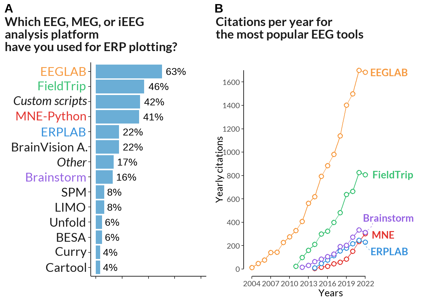
tools <- rev(c("EEGLAB", "FieldTrip", expression(italic("Custom scripts")), "MNE-Python", "ERPLAB", "BrainVision A.",
           expression(italic("Other")), "Brainstorm", "SPM", "LIMO", "Unfold", "BESA", "Curry", "Cartool"))
chart <- data.frame(rowSums(t(software))) %>%  tibble::rownames_to_column(., "soft") %>%
    rename_at(vars(colnames(.)), ~ c("soft", "sum_scores"))   %>% 
    filter(sum_scores != 0) %>% 
      mutate(soft = ifelse(sum_scores > 8, as.character(soft), "Other")) %>% group_by(soft) %>% 
      dplyr::summarise(sum_scores = sum(sum_scores)) %>% ungroup() %>% 
      mutate(percent_score = round(sum_scores / nrow(software) * 100))  %>% 
  mutate(soft = factor(soft, levels = soft[rev(order(sum_scores))])) %>% 
    ggplot(data = ., aes(y = reorder(soft, percent_score),  x= percent_score)) +
    geom_bar(stat="identity", fill ="#6BAED6") + 
    labs(x="",title="Which EEG, MEG, or iEEG analysis platform\nhave you used for ERP plotting?") +
    geom_text(aes(label = paste0(percent_score, "%")), 
            hjust = -0.2, size = 4)  + 
    theme_classic() + theme(
      axis.text.y = element_text(size = 14),
      legend.position="none", plot.caption.position = "plot", 
      plot.caption = element_text(hjust=0), 
      text = element_text(family = "Lato"),
      axis.text.x = element_blank(), axis.text = element_text(size = 10),  
      plot.title = element_text(color = "grey10", size = 16, face = "bold"),
      axis.title.y = element_blank(),
      #axis.title.x = element_blank(),
      plot.title.position = "plot"
      ) + 
    xlim(0, 100) +
    scale_y_discrete(labels = tools)

cbPalette <- rev(c("#e3342f",  "#38c172", "#3490dc", "#f6993f","#9561e2"))
cit_plot <- cit_data %>% filter(year < 2023) %>% group_by(year) %>% 
  mutate(ylast = case_when(year == 2022 ~ citations, TRUE ~ NA)) %>% 
  ggplot(., aes(x = year, y = citations, color = name, label = name)) + geom_line() +
  geom_point(shape = 21, fill = 'white', size=2, stroke=1) + 
  scale_color_manual(values=cbPalette) +  
  theme(legend.position = "none",
        panel.background = element_blank(), panel.border = element_blank(), strip.background = element_blank(), 
        text = element_text(family = "Lato"),
        plot.title = element_text(color = "grey10", size = 16, face = "bold", margin = margin(t = 15)),
        plot.title.position = "plot",)+
  scale_x_continuous(
    expand = c(0, 0),
    limits = c(2003.8, 2023), 
    breaks = seq(2004, 2023, by = 3)
  ) + labs(
    title = "Citations per year for the most popular EEG tools", subtitle = "", x = "Years", y = "Yearly citations"
  ) + geom_rangeframe(color = "black") +
  scale_y_continuous(
    expand = c(0.04, 0),
    breaks = seq(0, 1800, by = 200)
  )+ coord_cartesian(xlim = c(2004, 2029), clip = "off")  + 
  geom_text_repel(
    aes(color = name, label = name, x = 2022, y = ylast,),
    family = "Lato",
    fontface = "bold",
    size = 4,
    direction = "y",
    xlim = c(2022.3, NA),
    hjust = 0,
    segment.size = .7,
    segment.alpha = .5,
    segment.linetype = "dotted",
    box.padding = .4,
    segment.curvature = -0.1,
    segment.ncp = 3,
    segment.angle = 20
  )

Code

cbPalette2 <- c("#f6993f",  "#38c172", "grey10", "#e3342f", "#3490dc", "grey10", "grey10", "#9561e2", rep("grey10", 6))

f7 <- ggarrange(chart + labs(title="Which EEG, MEG, or iEEG\nanalysis platform\nhave you used for ERP plotting?")+
            theme( axis.text.y = element_text(color = rev(cbPalette2), face = "bold"),
              plot.title = element_text(color = "grey10", size = 14, margin = margin(t = 15))), 
          
          cit_plot + labs(title = "Citations per year for\nthe most popular EEG tools") +
            theme(plot.title = element_text(color = "grey10", face = "bold", size = 14, margin = margin(t = 15)))+
            scale_x_continuous(limits = c(2003.8, 2023), breaks = seq(2004, 2023, by = 3)), 
          labels = c("A", "B"), align = 'h')
f7 

Code

ggsave("../figures_jpg/Figure 7.jpg", f7, units = "px", dpi=200, width = 1500, height = 916)

Figure 8

Code

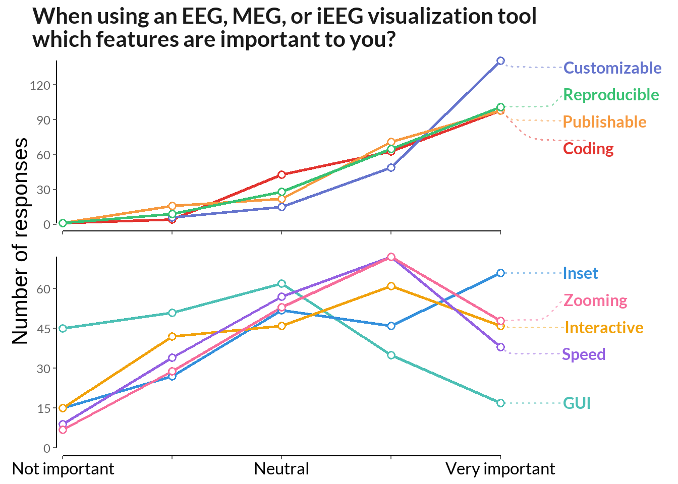
plot_features <- c(
  "Combine with a custom plot created outside of the toolbox (as subplot or inset)",
  "Flexible tweaking of plot attributes (colors, linewidths, margins etc.)",
  "Speed of plotting",
  "Presentation/publication ready figures",
  "Reproducibility of interactively generated or modified plots",
  "Zooming or panning within a plot",
  "Interactive selection of time-ranges or electrodes e.g. via Sliders or Dropdown menus",
  "Generating plots by clicking (GUI)",
  "Generating plots by coding"
)

feature1 <- data[52:60] %>% rename_all(., ~str_split_i(colnames(data[52:60]), "\\? \\[", 2) %>% str_sub(., 1, -2) ) %>%  
  mutate_at(c(colnames(.)), 
        funs(recode(.,
        "Very important"= 2, "Important"= 1, "Neutral"= 0,
        "Low importance"= -1, "Not at all important" = -2 ))) %>% 
  pivot_longer(cols = everything(), names_to = "name", values_to = "value") %>% 
  mutate(index = as.integer(factor(name))) %>% 
  filter(!is.na(value))

comb_data <- feature1 %>%  mutate(name = case_when(
  name == "Combine with a custom plot created outside of the toolbox (as subplot or inset)" ~ "Inset",
  name == "Flexible tweaking of plot attributes (colors, linewidths, margins etc.)"~ "Customizable",
  name == "Speed of plotting"~ "Speed",
  name == "Presentation/publication ready figures"~ "Publishable",
  name == "Reproducibility of interactively generated or modified plots"~ "Reproducible",
  name == "Zooming or panning within a plot"~ "Zooming",
  name == "Interactive selection of time-ranges or electrodes e.g. via Sliders or Dropdown menus"~ "Interactive",
  name == "Generating plots by clicking (GUI)"~ "GUI",
  name == "Generating plots by coding" ~ "Coding"
  )) %>% 
    mutate(gr = case_when(
      grepl("\\b(Speed|Zooming|GUI|Interactive)\\b", name) == TRUE ~ "Moderate",
      grepl("\\b(Coding|Customizable|Reproducible|Publishable|Inset)\\b", name) == TRUE ~ "Favored"))

test <-  comb_data %>% group_by(name, value) %>% dplyr::summarise(n = n()) %>% 
    mutate(gr = case_when(
      grepl("\\b(Speed|Zooming|GUI|Interactive|Inset)\\b", name) == TRUE ~ "Moderate",
      grepl("\\b(Coding|Customizable|Reproducible|Publishable)\\b", name) == TRUE ~ "Favored"))  %>% 
  mutate(denymax = case_when(value == 2 ~ n, TRUE ~ NA))

Code

cbPalette_fe1 <- c("#e3342f", "#6574cd", "#f6993f",  "#38c172" )
cbPalette_fe2 <- c("#4dc0b5", "#3490dc","#f1a20b", "#9561e2", "white", "#f66d9b")

core <- function(df){
  g <- ggplot(data = df, aes(x = value, y = n, label = name, color = name)) + 
  geom_line(bw = 0.5, size = 1) + 
  geom_point(shape = 21, fill = 'white', size=2, stroke=1)+ 
  labs(x = "Values on the Likert scale", y = "Scores")  +  geom_rangeframe(color = "black") +
  theme(
    panel.background = element_blank(), panel.border = element_blank(), 
    legend.position = "none", 
    text = element_text(family = "Lato"),
    strip.background = element_blank(), 
    axis.text = element_text(color = "grey40"),
    axis.ticks = element_line(color = "grey40", size = .5),
    strip.text = element_text(size = 14),
    axis.title = element_blank(),
    plot.title = element_text(
      color = "grey10", 
      size = 16, 
      face = "bold",
      ),
    plot.title.position = "plot",
  )  +
  coord_cartesian(xlim = c(1, 6.5), clip = "off") +
  geom_text_repel(
    aes(color = name, label = name, x = 5, y = denymax,),
    family = "Lato",
    fontface = "bold",
    size = 4,
    direction = "y",
    xlim = c(5.5, NA),
    hjust = 0,
    segment.size = .7,
    segment.alpha = .5,
    segment.linetype = "dotted",
    box.padding = .4,
    segment.curvature = -0.1,
    segment.ncp = 3,
    segment.angle = 20
  ) 
  return(g)
} 

test1 <- test %>% filter(gr == "Favored") %>% mutate(value = value + 3) %>% 
  core(.) +
  scale_x_continuous(
    expand = c(0.01, 0),
    limits = c(0.9, 5), 
    breaks = seq(1, 5, by = 1)
  ) +
  scale_y_continuous(
    expand = c(0.04, 0),
    limits = c(0, NA),
    breaks = seq(0, 150, by = 30)
  ) +
  scale_color_manual(values = cbPalette_fe1) + theme(axis.text.x=element_blank()) +
  labs(title = "When using an EEG, MEG, or iEEG visualization tool\nwhich features are important to you?")  


test2 <- test %>% filter(gr != "Favored") %>% mutate(value = value + 3) %>% ungroup() %>% 
  tibble::add_row(name = "void", value = 1, n = 0, gr = "a", denymax=0) %>% 
  # line above is just to extend yaxis to zero
   core(.) +
  scale_x_continuous(
    expand = c(0.01, 0),
    limits = c(0.9, 5), 
    breaks = seq(1, 5, by = 1),
    
    labels = c("Not important", "", "Neutral", "", "Very important")
  ) +
  scale_y_continuous(
    expand = c(0.04, 0),
    limits = c(0, NA),
    breaks = seq(0, 72, by = 15)
  ) + 
  scale_color_manual(values = cbPalette_fe2) + theme(axis.text.x = element_text(color = "black", size = 12))

figure <- ggarrange(test1, test2, align = 'v', nrow = 2) 
require(grid)
f8 <- annotate_figure(figure, left = textGrob("Number of responses", rot = 90, vjust = 1, gp = gpar(cex = 1.3)))
f8

Code

ggsave("../figures_jpg/Figure 8.jpg", f8, units = "px", dpi=200, width = 1700, height = 916, bg = "white")

Figure 9

Code

bl2 <- table(abs(just[2] %>% na.omit() %>% rbind(data[77] %>% dplyr::rename(num = !!names(.)[1]) , .))) %>% data.frame() %>%  dplyr::rename(baseline = !!names(.)[1]) %>% 
  mutate(baseline = ifelse(Freq > 2, paste0("-", as.character(baseline)), "Other")) %>%
  dplyr::group_by(baseline) %>% dplyr::summarise(Freq = sum(Freq)) %>% 
  mutate(percent_score = round(Freq / sum(Freq), 2) *100) %>% arrange(desc(baseline)) %>% 
  mutate(baseline = factor(baseline, 
  levels = c("-500", "-300", "-250", "-200", "-100", "Other")))

italised1 <- c("-500", "-300", "-250", "-200", "-100", expression(italic("Other")))

periods_plot2 <- bl2 %>%
    ggplot(data = ., aes(x = baseline, y = percent_score)) +
    geom_bar(stat="identity", fill ="#6BAED6", width = 0.6) + 
  labs(x = "Recomended baseline duration\n(msec)", y = "") +  
  scale_y_continuous(breaks=seq(0, 60, 5)) + theme_classic() +
  theme(legend.position="none", plot.title = element_text(hjust = 0.5), text = element_text(family = "Lato")) +
  geom_text(aes(label = paste0(percent_score, "%"), group = baseline), position = position_dodge(width = .9), vjust = -0.3)   +
    theme(legend.position="none", plot.caption = element_text(hjust=0), axis.text.y = element_blank(), axis.text = element_text(size = 10)) + 
  scale_x_discrete(labels = italised1)

cv <- data %>% select(23, 24) %>% 
  rename_at(vars(colnames(.)), ~ c("measure", "analyse")) %>% 
  filter(measure < 10000, analyse < 500)  %>% 
  mutate(rate = round(analyse / measure, 2)) %>% 
  group_by(rate) %>% dplyr::summarise(n = n()) %>% 
  mutate(p = round(n / sum(n), 2))

an_me_plot <- cv %>%  
  ggplot(aes(x=rate, y = p)) + 
  geom_col(position = "identity", bins=300, fill ="#6BAED6") + 
  labs(x ="Ratio of electrodes\nanalysed / measured", y = "") +
  theme_classic() +
  theme(legend.position="none", plot.caption = element_text(hjust=0), text = element_text(family = "Lato"), axis.text = element_text(size = 10)) + 
  #ylim(0, 0.1) + 
  scale_x_continuous(labels = scales::percent)  + scale_y_continuous(labels = scales::percent, limits = c(0, 0.4)) +
   labs(y = "Percentage of respondents")

Code

f9 <- ggarrange(periods_plot2 + labs(y = "Percentage of respondents")+ theme(axis.title.y = element_text(margin = margin (r = 10))), 
          an_me_plot + theme(axis.title.y = element_text(margin = margin (r = 10))), labels = c("A", "B")) 
f9

Code

ggsave("../figures_jpg/Figure 9.jpg", f9, units = "px", dpi=200, width = 1700, height = 916, bg = "white")

Figure 10

Code

t <- foreach(i = 1:nrow(data)) %do% tokenize_words(as.character(data[i, 11]))
tt <- foreach(i = 1:length(t)) %do% paste(unlist(t[i]), collapse = ' ') 

area1 <- data.frame(matrix(tt)) %>% dplyr::rename(words = !!names(.)[1]) %>%
  mutate(words = ifelse(str_detect(.[[1]], 'emot|empathy'), "affective neuroscience", words)) %>%  
  mutate(words =ifelse(str_detect(.[[1]], 'memory'), "memory", words)) %>% 
  mutate(words =ifelse(str_detect(.[[1]], 'hearing|audit'), "auditory", words)) %>% 
  mutate(words =ifelse(str_detect(.[[1]], 'cognitive load|selective attention|attention|cognition|consciousness|meditation|cognitive control|self|executive functions'), "attention", words)) %>% 
  mutate(words =ifelse(str_detect(.[[1]], 'dbs'), "deep brain stimulation", words)) %>% 
  mutate(words =ifelse(str_detect(.[[1]], 'decision making|reward'), "decision making", words)) %>%
  mutate(words =ifelse(str_detect(.[[1]], 'ageing'), "ageing", words)) %>% 
  mutate(words =ifelse(str_detect(.[[1]], 'social'), "social cognition", words)) %>% 
  mutate(words =ifelse(str_detect(.[[1]], 'olfac'), "olfaction", words)) %>% 
  mutate(words =ifelse(str_detect(.[[1]], 'communication|language|speech|biling|english|language processing'), "language and speech", words)) %>% 
  mutate(words =ifelse(str_detect(.[[1]], 'bci'), "bci", words)) %>% 
  mutate(words =ifelse(str_detect(.[[1]], 'sleep'), "sleep", words)) %>% 
  mutate(words =ifelse(str_detect(.[[1]], 'timing|time|temporal'), "time", words)) %>% 
  mutate(words =ifelse(str_detect(.[[1]], 'perception'), "perception", words)) %>% 
  mutate(words =ifelse(str_detect(.[[1]], 'vis'), "vision", words)) %>% 
  mutate(words =ifelse(str_detect(.[[1]], 'developmental|development|ageing'), "development", words)) %>% 
  mutate(words =ifelse(str_detect(.[[1]], 'spatial|brain body|motor|motion'), "motor control", words)) %>% 
  mutate(words =ifelse(str_detect(.[[1]], 'diagnostics|disorder|psychiatry|epilepsy|autism|patients|therapy|psychopharmacology'), "mental disorders", words)) %>%   
  mutate(words =ifelse(str_detect(.[[1]], 'signal processing|event related potentials|method|sdf|ieeg'), "dsp", words))

area <- area1 %>%
  mutate(words = ifelse(str_detect(.[[1]], 'olfaction|vision|auditory|pain'), "perception", words))%>%
  mutate(words = ifelse(str_detect(.[[1]], 'dsp|computational neuroscience'), "methodology", words)) %>% 
  mutate(words = ifelse(str_detect(.[[1]], 'mental disorders|deep brain stimulation'), "clinical", words))%>% 
  mutate(words = ifelse(str_detect(.[[1]], 'social cognition'), "affective neuroscience", words))

colours = c("#f9a65a", "#599ad3")
ud <- table(data[79]) %>% data.frame() %>% 
  rename_at(vars(colnames(.)), ~ c("position", "scores")) %>%
  mutate(percent_score = round(scores / sum(scores) * 100)) 

as <- cbind(unlist(area$words), unlist(data[[79]])) %>% data.frame() %>% 
filter(.[[2]] != "NANA") %>% dplyr::rename(area=X1, ud=X2) %>%
group_by(area) %>%
filter(n() > 2) %>% group_by(area, ud) %>% dplyr::summarise(n = n()) %>% 
  group_by(area) %>% dplyr::mutate(nn = sum(n)) %>% filter(area != "")

f10 <- as %>% 
  ggplot(., aes(x = n, y = reorder(area, nn), fill = ud)) +
  geom_col(stat = "identity", width = 0.7) + 
  labs(x = "Percentage of respondents", y = "", fill ="Positive:", title = "In ERP plots, should positive voltages\nbe plotted upwards, or downwards?") +
  theme_classic()+
  geom_text(aes(label = n, group = ud), 
            position = position_stack(vjust = 0.5), size = 4)  +
  coord_cartesian(clip = "off") +
  theme(axis.text = element_text(size = 12),
        text = element_text(family = "Lato"),
        axis.title = element_text(size = 12),
        title = element_text(size = 14),
        axis.title.y=element_blank(),
        
        legend.title = element_blank(),
        legend.direction = "horizontal",
        legend.position = c(0.8, 0.2),
        
        plot.title.position = "plot",
        plot.caption.position = "plot",
        ) +  
  scale_fill_manual(values=colours, limits = c("Up", "Down")) +
  scale_x_continuous(labels = scales::percent_format(scale = 1, accuracy = 1))

f10

Code

ggsave("../figures_jpg/Figure 10.jpg", f10, units = "px", dpi=200, width = 1700, height = 916, bg = "white")
ggsave("../figures_png/Figure 10.png", f10, units = "px", dpi=200, width = 1700, height = 916, bg = "white")

Code

area_short <- area %>% 
  mutate(words = ifelse(str_detect(.[[1]], 'language and speech|attention'), 
                        "language, speech,\nattention", 
                        "affective neuroscience,\nbci, clinical, decision making,\ndevelopment, memory,\nmethodology, motor control,\nperception, sleep, time")) 

as2 <- cbind(unlist(area_short$words), unlist(data[[79]])) %>% data.frame() %>% 
filter(.[[2]] != "NANA") %>% dplyr::rename(area=X1, ud=X2) %>%
group_by(area) %>%
filter(n() > 2) %>% group_by(area, ud) %>% dplyr::summarise(n = n()) %>% 
  group_by(area) %>% dplyr::mutate(nn = sum(n)) %>% filter(area != "") %>% 
  dplyr::mutate(n = round(n / 199 *100), nn = round(nn / 199 * 100))

f10_2 <- as2 %>% 
  ggplot(., aes(x = n, y = reorder(area, nn), fill = ud)) +
  geom_col(stat = "identity", width = 0.7) +
  labs(x = "Percent of respondents", y = "", fill ="Positive:", title = "In ERP plot, should positive voltages\nbe plotted upwards, or downwards?") +
  theme_classic()+
  geom_text(aes(label = paste0(n, "%"), group = ud), 
            position = position_stack(vjust = 0.5), size = 4)  +
  coord_cartesian(clip = "off") +
  theme(axis.text = element_text(size = 12),
        text = element_text(family = "Lato"),
        axis.title = element_text(size = 12),
        title = element_text(size = 14),
        axis.title.y=element_blank(),
        
        legend.title = element_blank(),
        legend.direction = "horizontal",
        legend.position = c(0.8, 0.2),
        
        plot.title.position = "plot",
        plot.caption.position = "plot",
        ) +  
  scale_fill_manual(values=colours, limits = c("Up", "Down")) 

f10_2 

Code

ggsave("../figures_jpg/Figure 10_2.jpg", f10_2, units = "px", dpi=200, width = 1700, height = 916, bg = "white")
ggsave("../figures_png/Figure 10_2.png", f10_2, units = "px", dpi=200, width = 1700, height = 916, bg = "white")

Code

f10_3 <- as2 %>% 
  ggplot(., aes(y = n, x = reorder(area, nn), fill = ud)) +
  geom_col(stat = "identity", width = 0.3) +
  labs(y = "Percent of respondents", x = "", fill ="Positive:", title = "In ERP plot, should positive voltages\nbe plotted upwards, or downwards?") +
  theme_classic()+
  geom_text(aes(label = paste0(n, "%"), group = ud), 
            position = position_stack(vjust = 0.5), size = 4)  +
  coord_cartesian(clip = "off") +
  theme(axis.text = element_text(size = 12),
        text = element_text(family = "Lato"),
        axis.title = element_text(size = 12),
        title = element_text(size = 14),
        
        legend.title = element_blank(),
        legend.position = c(0.95, 0.2),
        aspect.ratio = 0.5/1,
        
       # plot.title.position = "plot",
       # plot.caption.position = "plot",
        ) +  
  scale_fill_manual(values=colours, limits = c("Up", "Down")) 


f10_3 

Code

ggsave("../figures_jpg/Figure 10_3.jpg", f10_3, units = "px", dpi=200, width = 1700, height = 916, bg = "white")

Figure 11

Code

eb <- table(data[74]) %>% data.frame() %>% rename_at(vars(colnames(.)), ~ c("Position", "Scores")) %>% 
  filter(Position != "Never published this plot") %>% 
  mutate(percent_score = round(Scores / sum(Scores) * 100)) 

eb_fig <- eb %>% 
    ggplot(., aes(y = Position, x = percent_score)) +
    geom_bar(stat = "identity", width=0.5, position = "dodge", fill ="#6BAED6") + theme_classic() +
  theme(axis.text.x = element_blank(),
        axis.title.y = element_blank(),
        legend.position="none", 
        text = element_text(family = "Lato"),
        axis.text = element_text(size = 12),
        plot.title = element_text(hjust = 0.5)) +
  geom_text(aes(label = paste0(percent_score, "%"), group = Position), 
            hjust = -0.2) + 
  ggtitle("In your paper, have you published\nan ERP plot with error bars?")+
scale_fill_manual(values=colours)  +
    theme(legend.position="none", plot.caption = element_text(hjust=0), axis.text = element_text(size = 10)) + 
  xlim(0, 100) + labs(y = "")

ebd <- data[75] %>%  filter(!is.na(.)) %>% table()  %>% data.frame() %>% rename_at(vars(colnames(.)), ~ c("position", "scores")) %>% mutate(percent_score = round(scores / sum(scores) * 100)) %>% filter(position != "Other") 

ebd_fig <- ebd %>% 
    ggplot(., aes(y = position, x = percent_score)) + 
    geom_bar(position = "dodge", stat = "identity", width=0.5, fill ="#6BAED6") + 
    theme_classic() +
    theme(axis.text.x = element_blank(), 
          text = element_text(family = "Lato"),
          legend.position="none", 
          axis.title.y = element_blank(),
          plot.title = element_text(hjust = 0.5)) + 
     
  geom_text(aes(label = paste0(percent_score, "%"), group = position),  hjust = -0.2) + 
  ggtitle("In your figure, what\ndid the error bars represent?")+
  scale_fill_manual(values=colours) + 
  scale_y_discrete(labels = c("Standard error\nof the mean", "Confidence\ninterval")) +
    theme(plot.caption = element_text(hjust=0), axis.text = element_text(size = 10)) + xlim(0, 100) 

f11 <- ggarrange(eb_fig + labs(x = "Percentage of respondents"), ebd_fig + labs(x = "Percentage of respondents"),  
          labels = c("A", "B"),
          ncol = 2, nrow = 1, align = 'h') 
f11

Code

ggsave("../figures_jpg/Figure 11.jpg", f11, units = "px", dpi=250, width = 1700, height = 465, bg = "white")

Sup figure 2

Code

marg <- data %>% select(23, 24) %>% 
  rename_at(vars(colnames(.)), ~ c("Recorded", "Analysed")) %>% 
  filter(Recorded < 10000, Analysed < 500)   %>%  
  ggplot(., aes(y=Analysed, x = Recorded)) + geom_point() +
      theme(legend.position="none") + theme_classic() + labs(x = "Electrodes recorded", y = "Electrodes aanlysed") 
sf2 <- ggMarginal(marg, type="histogram") 
sf2