Software usage

Here we present researcher’s visualization customs and awareness about some methodological problems.

Setup

[1] TRUE

Code

data <- read_excel("../data/results_survey.xlsx") #change to csv or tab and check will it work

data <- data[1:121] %>% 
  filter(.[[18]] !='Yes') # not analysed any EEG method

Code

cit1 <- read.table(file = "../data/cit/eeglab.txt", header = TRUE, fill = TRUE)[1:2] %>% mutate(name = "EEGLAB")
cit2 <- read.table(file = "../data/cit/mne.txt", header = TRUE, fill = TRUE)[1:2]%>% mutate(name = "MNE")
cit3 <- read.table(file = "../data/cit/erplab.txt", header = TRUE, fill = TRUE)[1:2]%>% mutate(name = "ERPLAB")
cit4 <- read.table(file = "../data/cit/fieldtrip.txt", header = TRUE, fill = TRUE)[1:2]%>% mutate(name = "FieldTrip")
cit5 <- read.table(file = "../data/cit/brainstorm.txt", header = TRUE, fill = TRUE)[1:2]%>% mutate(name = "Brainstorm")

cit_data <- rbind(cit1, cit2, cit3, cit4, cit5) %>% rename_at(vars(colnames(.)), ~ c("year", "citations", "name"))

Software usage

Frequency

Code

na.omit(data[51]) %>% nrow()

[1] 22

Code

other <- c(rep("Custom scripts", each=9), "4DBTi", rep("letswave", 3), "mTRF", "RAGU", "IGOR Pro", "EEGProcessor", "ELAN", "WinEEG") %>% table(.) %>% data.frame(.) %>% rename_at(vars(colnames(.)), ~ c("soft", "sum_scores"))

Code

vec <- names(data[25:50]) %>% str_split_i(., "\\? \\[", 2) %>%  str_sub(., 1, -2)

software <- data[25:50] %>%
    rename_at(vars(colnames(.)), ~ vec) %>% 
  mutate_at(vars(vec), function(., na.rm = FALSE) (x = ifelse(.=="Yes", 1, 0))) %>% 
  cbind(., data[51] %>% rename_at(vars(colnames(.)), ~ c("other"))) %>% mutate(other = case_when(
      grepl("\\b(letswave)\\b", other, ignore.case = TRUE) == TRUE ~ "Letswave",
      grepl("\\b(r|matlab|python|ggplot(2)?|own)\\b", other, ignore.case = TRUE) == TRUE ~ "Custom scripts",
      grepl("\\bnever\\b", other, ignore.case = TRUE) == TRUE ~ NA_character_,
      TRUE ~ as.character(other)
      ))  %>%
  mutate(cs = ifelse(other == "Custom scripts", other, NA_character_),
         other2 = ifelse(other != "Custom scripts", other, NA_character_)) %>% 
  mutate(`Custom scripts` = case_when(
    cs == "Custom scripts" ~ as.numeric(1),
    TRUE ~ as.numeric(`Custom scripts`)
  )) %>% 
  mutate(Letswave = case_when( #gross
    other2 == "Letswave" ~ as.numeric(1),
    TRUE ~ as.numeric(0)
  )) %>% dplyr::select(-cs, -other, -other2) # next time I also will extend other 2 too


d <- data.frame(rowSums(t(software))) %>%  tibble::rownames_to_column(., "soft") %>% 
    rename_at(vars(colnames(.)), ~ c("soft", "sum_scores"))   %>% 
    filter(sum_scores != 0) %>% 
      mutate(soft = ifelse(sum_scores > 8, as.character(soft), "Other")) %>% group_by(soft) %>% 
      dplyr::summarise(sum_scores = sum(sum_scores)) %>% ungroup() %>% 
      mutate(percent_score = round(sum_scores / nrow(software) * 100))  %>% 
  mutate(soft = factor(soft, levels = soft[rev(order(sum_scores))]))

Code

tools <- rev(c("EEGLAB", "FieldTrip", expression(italic("Custom scripts")), "MNE-Python", "ERPLAB", "BrainVision A.",
           expression(italic("Other")), "Brainstorm", "SPM", "LIMO", "Unfold", "BESA", "Curry", "Cartool"))

chart <- d %>% 
    ggplot(data = ., aes(y = reorder(soft, percent_score),  x= percent_score)) +
    geom_bar(stat="identity", fill ="#6BAED6") + 
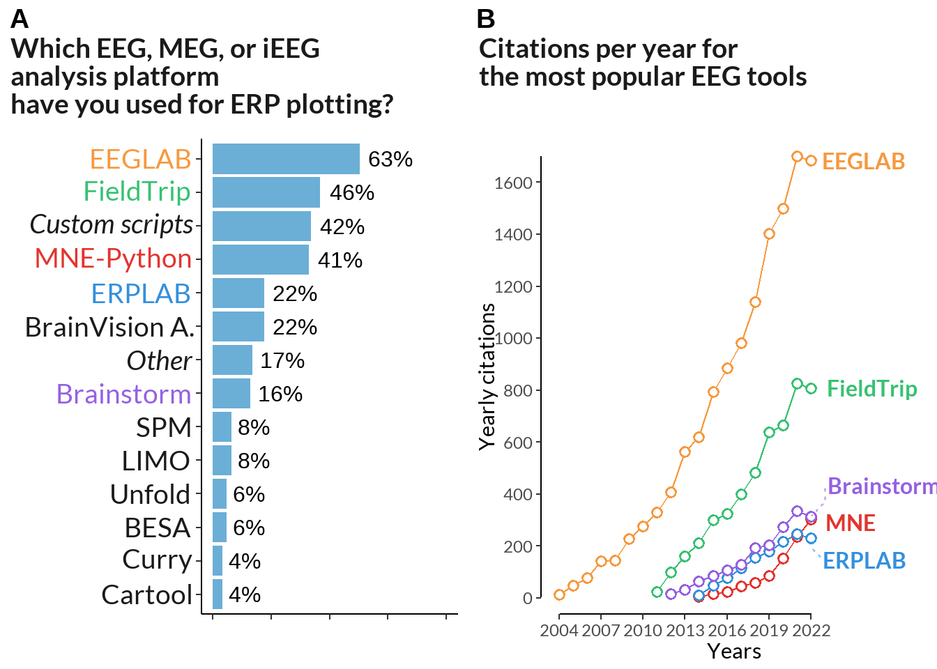
    labs(x="",title="Which EEG, MEG, or iEEG analysis platform\nhave you used for ERP plotting?") +
    geom_text(aes(label = paste0(percent_score, "%")), 
            hjust = -0.2, size = 4)  + 
    theme_classic() + theme(
      axis.text.y = element_text(size = 14),
      legend.position="none", plot.caption.position = "plot", 
      plot.caption = element_text(hjust=0), 
      text = element_text(family = "Lato"),
      axis.text.x = element_blank(), axis.text = element_text(size = 10),  
      plot.title = element_text(color = "grey10", size = 16, face = "bold"),
      axis.title.y = element_blank(),
      #axis.title.x = element_blank(),
      plot.title.position = "plot"
      ) + 
    xlim(0, 100) +
    scale_y_discrete(labels = tools)

chart +
    labs(caption = sprintf("N of respondents - %d",  nrow(software)))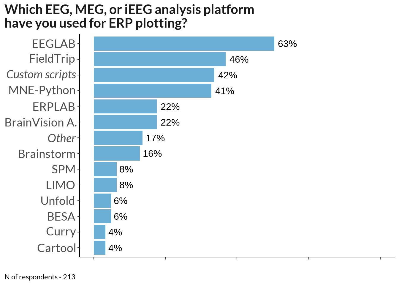

Matlab users

Code

data.frame(rowSums(t(software))) %>%  tibble::rownames_to_column(., "soft") %>% 
    rename_at(vars(colnames(.)), ~ c("soft", "sum_scores"))   %>% 
    filter(sum_scores != 0) %>% 
   mutate(soft = case_when(
      grepl("\\b(EEGLAB|FieldTrip|ERPLAB|Brainstorm)\\b", soft) == TRUE ~ "MATLAB-based tools", 
      TRUE ~ soft
      )) %>% 
      #mutate(soft = ifelse(sum_scores > 8, as.character(soft), "Other")) %>% 
  group_by(soft) %>% 
      dplyr::summarise(sum_scores = sum(sum_scores)) %>% ungroup() %>% 
      mutate(percent_score = round(sum_scores / nrow(software) * 100))  %>% 
  mutate(soft = factor(soft, levels = soft[rev(order(sum_scores))])) %>% 
  arrange(desc(sum_scores)) %>% head(5)

# A tibble: 5 × 3
  soft                    sum_scores percent_score
  <fct>                        <dbl>         <dbl>
1 "MATLAB-based tools"           313           147
2 "Custom scripts"                90            42
3 "MNE-Python"                    88            41
4 "Brain Vision Analyser"         47            22
5 "SPM "                          18             8

Code

software %>% select(EEGLAB, FieldTrip, ERPLAB, Brainstorm) %>% mutate(sum = rowSums(across(where(is.numeric)))) %>% 
    filter(sum != 0) %>% summarise(n = n()/ nrow(software) * 100)

         n
1 82.62911

Monousers

Soft frequency among those who used only one software

Code

ns <- cbind(data.frame(rowSums(software), software)) %>% 
  filter(rowSums.software. == 1) %>% dplyr::select(-rowSums.software.)

data.frame(rowSums(t(ns))) %>%  
  tibble::rownames_to_column(., "soft") %>% 
   rename_at(vars(colnames(.)), ~ c("soft", "sum_scores")) %>% 
  arrange(., desc(sum_scores)) %>% filter(sum_scores != 0)

                   soft sum_scores
1            MNE.Python         11
2                EEGLAB          9
3             FieldTrip          8
4 Brain.Vision.Analyser          2
5        Custom.scripts          2
6                ERPLAB          1
7                  SPM.          1
8                Unfold          1

Number of used tools

Code

nu_med <- data.frame(rowSums(software)) %>%  dplyr::rename(n_soft = rowSums.software.) %>% summarise(median_n_soft = median(n_soft)) %>% as.numeric()

data.frame(rowSums(software)) %>%  dplyr::rename(n_soft = rowSums.software.) %>% #arrange(desc(n_soft))
 ggplot(data = ., aes(n_soft)) +
  geom_histogram(bins = 45) +  scale_x_continuous(breaks=seq(0, 30, 1)) +
  labs(x ="Number of software used", y="Count") +
  theme_classic() + theme(legend.position="none", axis.text.x = element_text(size = 12))  +
    labs(caption = sprintf("N of respondents - %d, median - %d",  nrow(software), nu_med)) +
    theme(legend.position="none", plot.caption = element_text(hjust=0), axis.text = element_text(size = 10))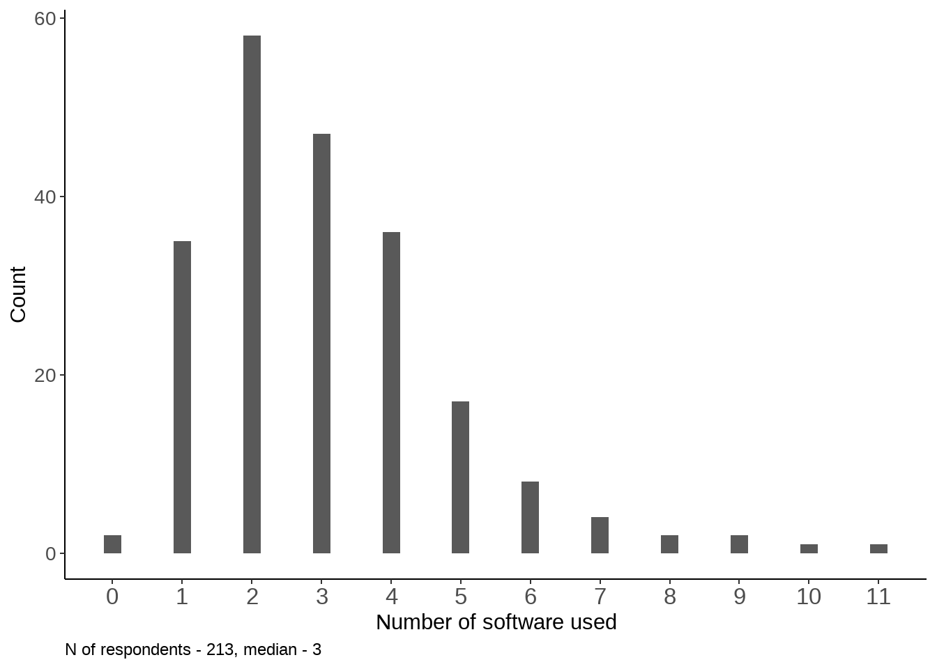 

Cooccurrence

Code

library(reshape2)
# how to order by diagonal matrix 
# how to add others
software <- data[25:50]
d1 <- foreach(i = colnames(software)) %do% ifelse(software[i]=="Yes", 1, 0)
c <- crossprod(matrix(unlist(d1), ncol = 26))
rownames(c) <- colnames(software) %>% str_split_i(., "\\? \\[", 2) %>%  str_sub(., 1, -2)
colnames(c) <- rownames(c)

diag.order <- order(diag(c), decreasing = FALSE)
mat_reordered <- c[diag.order, diag.order]

mat_reordered %>%  reshape2::melt(.) %>% ggplot(., aes(x=Var1, y=Var2)) + 
  geom_tile(aes(fill = value)) + 
  geom_text(aes(label = value)) +
  scale_fill_gradient(low = "white", high = "red") +
  theme(legend.title = element_blank(),
        axis.title=element_blank(),
        axis.text.x = element_text(angle = 90, vjust = 1, hjust=1)) +
    labs(caption = sprintf("N of respondents - %d",  nrow(software))) +
    theme(legend.position="none", plot.caption.position = "plot", plot.caption = element_text(hjust=0), axis.text = element_text(size = 10))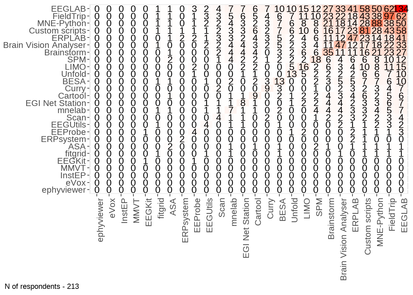 

Code

zero_rows <- rowSums(mat_reordered) == 0
zero_cols <- colSums(mat_reordered) == 0

# Create a new matrix array without the rows and columns consisting only of zeroes
new_matrix <- mat_reordered[!zero_rows, !zero_cols]
new_matrix %>% reshape2::melt(.) %>% ggplot(., aes(x=Var1, y=Var2)) + 
  geom_tile(aes(fill = value)) + 
  geom_text(aes(label = value)) +
  scale_fill_gradient(low = "white", high = "red") +
  theme(legend.title = element_blank(),
        axis.title=element_blank(),
        axis.text.x = element_text(angle = 90, vjust = 1, hjust=1)) +
    labs(caption = sprintf("N of respondents - %d. Zero rows are excluded",  nrow(software))) +
    theme(legend.position="none", plot.caption.position = "plot", plot.caption = element_text(hjust=0), axis.text = element_text(size = 10))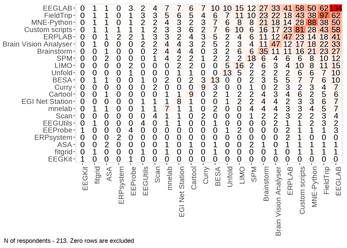 

Software usage based on citations

Code

cbPalette <- rev(c("#e3342f",  "#38c172", "#3490dc", "#f6993f","#9561e2"))
#font_add_google("Lato")

#showtext_opts(dpi = 100)
#showtext_auto(enable = TRUE)

cit_plot <- cit_data %>% filter(year < 2023) %>% group_by(year) %>% 
  mutate(ylast = case_when(year == 2022 ~ citations, TRUE ~ NA)) %>% 
  ggplot(., aes(x = year, y = citations, color = name, label = name)) + geom_line() +
  geom_point(shape = 21, fill = 'white', size=2, stroke=1) + 
  scale_color_manual(values=cbPalette) +  
  theme(legend.position = "none",
        panel.background = element_blank(), panel.border = element_blank(), strip.background = element_blank(), 
        text = element_text(family = "Lato"),
        plot.title = element_text(color = "grey10", size = 16, face = "bold", margin = margin(t = 15)),
        plot.title.position = "plot",)+
  scale_x_continuous(
    expand = c(0, 0),
    limits = c(2003.8, 2023), 
    breaks = seq(2004, 2023, by = 3)
  ) + labs(
    title = "Citations per year for the most popular EEG tools", subtitle = "", x = "Years", y = "Yearly citations"
  ) + geom_rangeframe(color = "black") +
  scale_y_continuous(
    expand = c(0.04, 0),
    breaks = seq(0, 1800, by = 200)
  )+ coord_cartesian(xlim = c(2004, 2029), clip = "off")  + 
  geom_text_repel(
    aes(color = name, label = name, x = 2022, y = ylast,),
    family = "Lato",
    fontface = "bold",
    size = 4,
    direction = "y",
    xlim = c(2022.3, NA),
    hjust = 0,
    segment.size = .7,
    segment.alpha = .5,
    segment.linetype = "dotted",
    box.padding = .4,
    segment.curvature = -0.1,
    segment.ncp = 3,
    segment.angle = 20
  )# 

cit_plot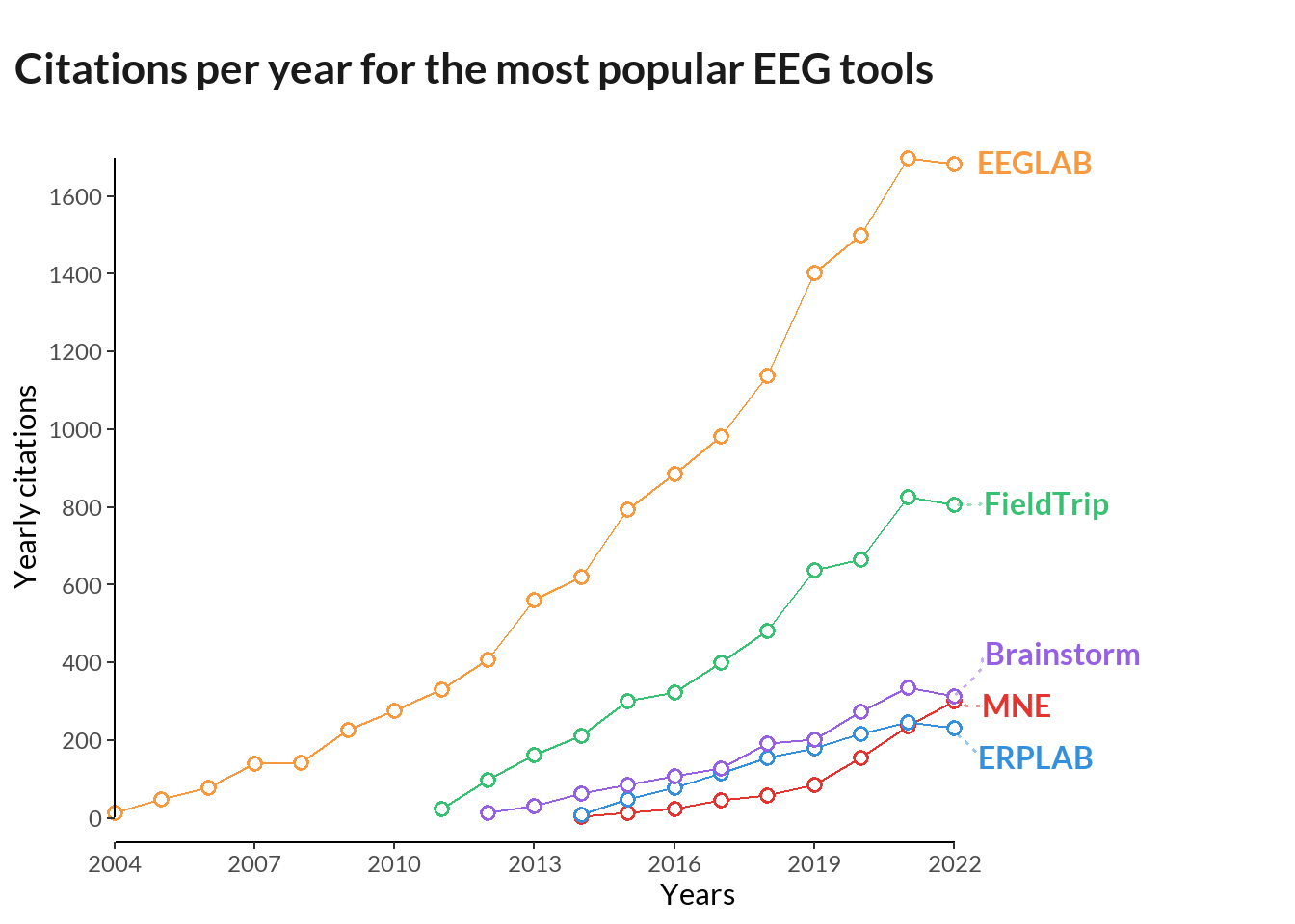

Comb

Code

#showtext_opts(dpi = 100)
#showtext_auto(enable = TRUE)
cbPalette2 <- c("#f6993f",  "#38c172", "grey10", "#e3342f", "#3490dc", "grey10", "grey10", "#9561e2", rep("grey10", 6) )
ggarrange(chart + labs(title="Which EEG, MEG, or iEEG\nanalysis platform\nhave you used for ERP plotting?")+
            theme( axis.text.y = element_text(color = rev(cbPalette2), face = "bold"),
              plot.title = element_text(color = "grey10", size = 14, margin = margin(t = 15))), 
          
          cit_plot + labs(title = "Citations per year for\nthe most popular EEG tools") +
            theme(plot.title = element_text(color = "grey10", face = "bold", size = 14, margin = margin(t = 15)))+
            scale_x_continuous(limits = c(2003.8, 2023), breaks = seq(2004, 2023, by = 3)), 
          labels = c("A", "B"), align = 'h')