Sample bio

Here we show a statistics about our study sample: biographical and experience data

Setup

Code

data <- read_excel("../data/results_survey.xlsx")
data <- data[1:121] %>% 
  filter(.[[18]] !='Yes') # not analysed any EEG method

font_add_google("Lato")
showtext_opts(dpi = 200)
showtext_auto(enable = TRUE)

Sample overview

Country

Code

country <- data.frame(table(data[8]))  %>% dplyr::rename(country_work = !!names(.)[1]) %>%
  mutate(country_work = ifelse(Freq >= 6, as.character(country_work), "Other")) %>% group_by(country_work) %>% 
  mutate(country_work = case_when(
    country_work == "United Kingdom" ~ "UK",
    TRUE ~ as.character(country_work)  
  )) %>% 
  dplyr::summarise(Freq = sum(Freq)) %>% 
  dplyr::mutate(percent_score = round(Freq / sum(Freq) * 100)) %>% 
  mutate(country_work = factor(country_work, levels = country_work[rev(order(percent_score))]))

italised1 <- rev(c("Germany", expression(italic("Other")), "USA", "UK", "France", "Netherlands", "Switzerland", "Spain", "Italy", "Russia", "Belgium", "Australia"))


country_fig <- country %>%
  ggplot(data = ., aes(y = reorder(country_work, percent_score),  x= percent_score)) +#, fill = country_work)) +
  geom_col(stat = "identity", width = 0.8) + 
  labs(x = "Percent", y="", title = "Country of work") +
  geom_text(aes(label = paste0(percent_score, "%")), hjust = -0.1,
  size = 4)  + theme_classic()   +
  theme(legend.position="none", 
        plot.caption.position = "plot", 
        plot.caption = element_text(hjust=0), 
        axis.text.y = element_text(size = 12),
        text = element_text(family = "Lato"),
        ) + coord_cartesian(clip = "off") +
    scale_y_discrete(labels = italised1)

country_fig + 
  labs(caption = sprintf("N of respondents = %d", sum(country$Freq)))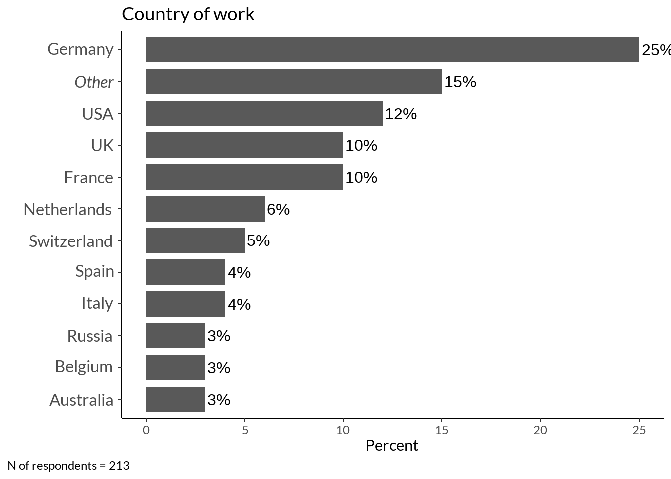 

Code

data.frame(table(data[8]))  %>% dplyr::rename(country_work = !!names(.)[1]) %>%
  #mutate(country_work = ifelse(Freq >= 6, as.character(country_work), "Others")) %>%
  group_by(country_work) %>% 
  mutate(country_work = case_when(
    country_work == "United Kingdom" ~ "UK",
    TRUE ~ as.character(country_work)  
  )) %>% 
  dplyr::summarise(Freq = sum(Freq)) %>% 
  dplyr::mutate(percent_score = round(Freq / sum(Freq) * 100)) %>% 
  mutate(country_work = factor(country_work, levels = country_work[rev(order(percent_score))])) %>% 
  arrange(desc(Freq))

# A tibble: 30 × 3
   country_work  Freq percent_score
   <fct>        <int>         <dbl>
 1 Germany         53            25
 2 USA             26            12
 3 France          22            10
 4 UK              22            10
 5 Netherlands     12             6
 6 Switzerland     10             5
 7 Spain            9             4
 8 Italy            8             4
 9 Russia           7             3
10 Australia        6             3
# ℹ 20 more rows

Code

c_df <- data.frame(table(data[8]))  %>% dplyr::rename(country_work = !!names(.)[1]) 
c_df$continent <- countrycode(sourcevar = c_df[, "country_work"],
                            origin = "country.name",
                            destination = "region23")
c_df %>% group_by(continent) %>% dplyr::summarise(Freq = sum(Freq)) %>%  ungroup() %>% 
  mutate(Per = round(Freq/ sum(Freq), 2) * 100) %>% 
  arrange(desc(Freq))

# A tibble: 14 × 3
   continent                  Freq   Per
   <chr>                     <int> <dbl>
 1 Western Europe              105    49
 2 Northern Europe              30    14
 3 Northern America             28    13
 4 Southern Europe              17     8
 5 Eastern Europe               11     5
 6 Australia and New Zealand     6     3
 7 Western Asia                  5     2
 8 Southern Asia                 3     1
 9 South America                 2     1
10 South-Eastern Asia            2     1
11 Central America               1     0
12 Central Asia                  1     0
13 Eastern Asia                  1     0
14 Western Africa                1     0

Field

Code

field <- as.data.frame(table(data[9])) %>% arrange(desc(Freq)) %>% head(3)
field$Freq[1] <- field$Freq[1] + 1 # from Others
field$Freq[2] <- field$Freq[2] + 1
field$Freq[3] <- field$Freq[3] + 1

fieldplot <- field %>% dplyr::rename(area = !!names(.)[1]) %>%
  mutate(percent_score = round(Freq / sum(Freq) * 100)) %>% 
    ggplot(data = ., aes(y = reorder(area, percent_score),  x = percent_score)) +
    geom_col(stat="identity", width = 0.7) + labs(y = "", title="Field of research", x ="Percent") +
    geom_text(aes(label = paste0(percent_score, "%")), hjust = -0.1)  + 
  theme_classic()  +
    theme(legend.position="none", 
          plot.caption = element_text(hjust=0), 
          text = element_text(family = "Lato"),
          axis.text.y = element_text(size = 12)) + scale_y_discrete(labels=c("Applied", "Clinical", "Fundamental")) + 
  coord_cartesian(clip = "off") #+ scale_fill_grey(start = .9, end = 0)
fieldplot + 
    labs(caption = sprintf("N of respondents = %d", sum(field$Freq)))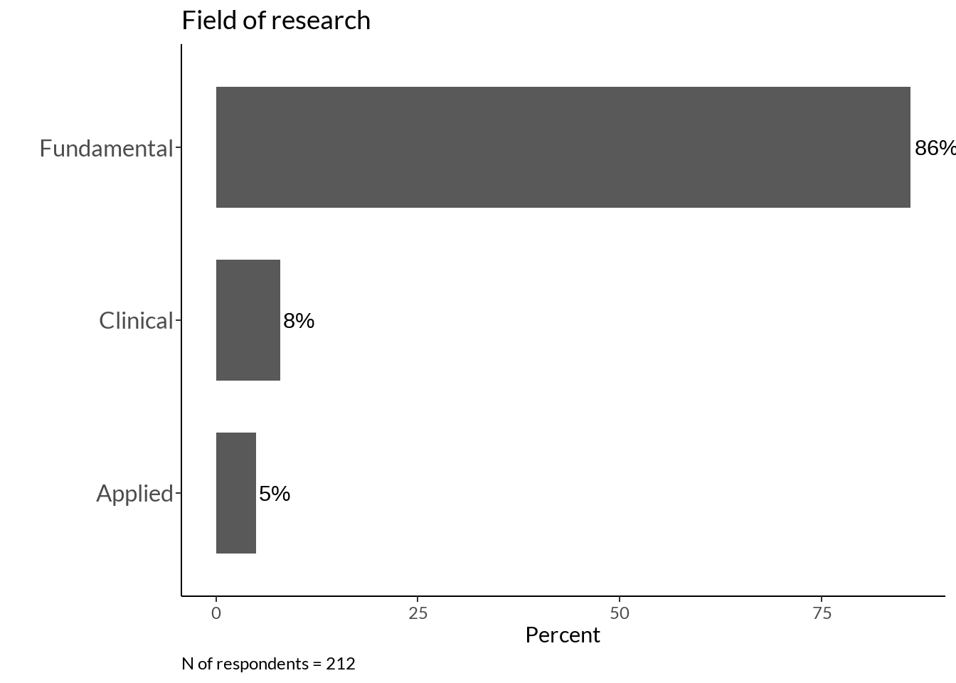

Position

Methods

Code

method <- data[14:17]
colnames(method) <- names(method) %>%  str_split_i(., "\\? \\[", 2)  %>%  str_sub(., 1, -2)

methods <- data.frame(rowSums(t(data.frame(foreach(i = colnames(method)) %do% ifelse(method[i]=="Yes", 1, 0))))) %>% 
  tibble::rownames_to_column(., "plots") %>% 
    dplyr::rename(method = !!names(.)[1], sum_scores = !!names(.)[2])  %>%  
    mutate(percent_score = round(sum_scores / sum(sum_scores) * 100)) %>% 
  
    ggplot(., aes(y = reorder(method, percent_score), x = percent_score)) + 
    geom_col(stat = "identity", width = 0.7) + labs(y = "", x = "Percent", title = "Method") +
    geom_text(aes(label = paste0(percent_score, "%")), hjust = -0.1)+
    theme_classic() + 
    theme(legend.position="none", text = element_text(family = "Lato"), 
          plot.caption = element_text(hjust=0), axis.text.y = element_text(size = 14)) +
    scale_y_discrete(labels=c("OPMs MEG", "Intracranial EEG", "SQUID MEG", "Scalp EEG")) +
    coord_cartesian(clip = "off") + xlim(0, 75)

methods + 
    labs(caption = sprintf("N of respondents = %d", nrow(method)))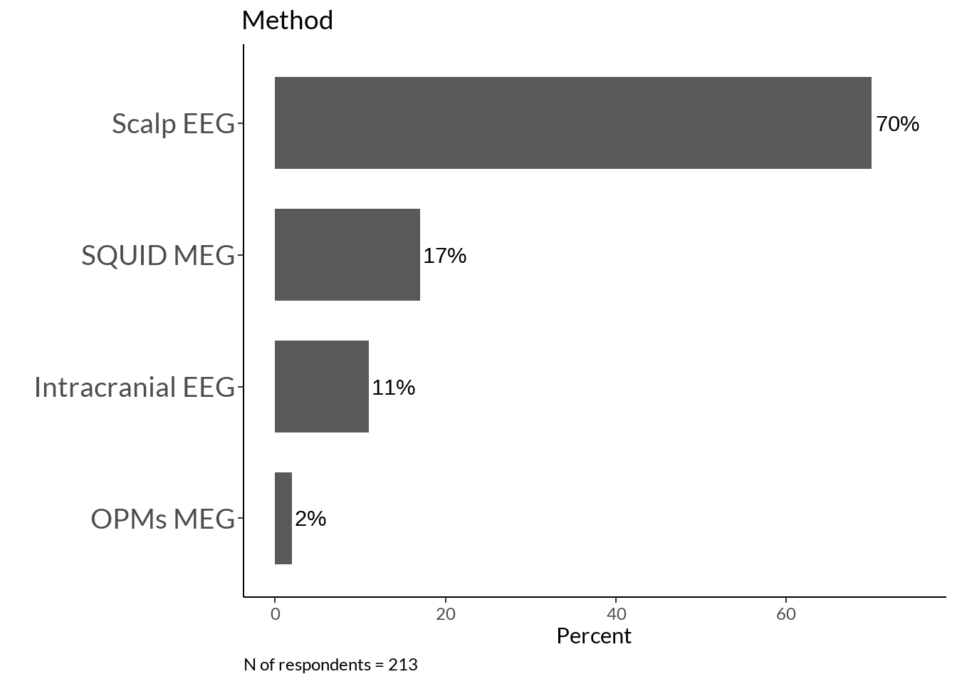

Topic

Code

t <- foreach(i = 1:nrow(data)) %do% tokenize_words(as.character(data[i, 11]))
tt <- foreach(i = 1:length(t)) %do% paste(unlist(t[i]), collapse = ' ') 

area <- data.frame(matrix(tt)) %>% dplyr::rename(words = !!names(.)[1]) %>%
   mutate(words2 = case_when(
    grepl("\\bmemory\\b", words) == TRUE ~ "memory", 
    grepl("\\b(empathy|emot\\w*|affective|social)\\b", words) == TRUE ~ "affective neuroscience", 
    grepl("\\b(cognitive load|selective attention|attention|cognition|consciousness|meditation|cognitive control|self|executive functions)\\b", words) == TRUE ~ "cognitive control and attention", 
    grepl("\\b(hearing|audi\\w*)\\b", words) == TRUE ~ "auditory",
    grepl("\\b(decision|reward)\\b", words) == TRUE ~ "decision making",
    grepl("\\b(ageing|aging)\\b", words) == TRUE ~ "ageing",
    grepl('\\bolfac\\w*', words) ~ 'olfaction',
    grepl('\\b(communication|language|speech|biling\\w*|english)\\b', words) ~ 'language and speech',
    grepl('\\bbci\\b', words) ~ 'bci',
    grepl('\\bsleep\\b', words) ~ 'sleep',
    grepl('\\b(timing|time|temporal)\\b', words) ~ 'time',
    grepl('\\bperception\\b', words) ~ 'perception',
    grepl('\\bvis\\w*', words) ~ 'vision',
    grepl('\\b(development\\w*|ageing)\\b', words) ~ 'development',
    grepl('\\b(spatial|brain body|motor|motion)\\b', words) ~ 'motor control',
    grepl('\\b(diagnostics|disorder(s)?|psychiatry|epilepsy|autism|patients|therapy|psychopharmacology|pain|dbs|stimulation)\\b', words) ~ 'mental disorders',
    grepl('\\b(signal|potentials|method\\w*|sdf|ieeg|computational)\\b', words) ~ 'methodology',
    grepl('\\b(olfaction|vision|auditory)\\b', words) ~ 'development',
    ))
   
area %>% group_by(words2) %>% dplyr::summarise(Freq = n()) %>% 
  data.frame(.)  %>% mutate(words2 = as.character(words2)) %>%  #arrange(desc(Freq)) %>% 
    ggplot(data = ., aes(y = reorder(words2, Freq),  x= Freq)) +
    geom_bar(stat="identity") + labs(x="Topic of research", y="Frequency") +
    geom_text(aes(label = Freq), 
    hjust = -0.2) + theme_classic() +
    labs(caption = sprintf("N of respondents = %d", nrow(area))) +
    theme(legend.position="none", plot.caption.position = "plot", plot.caption = element_text(hjust=0), axis.text.y = element_text(size = 11))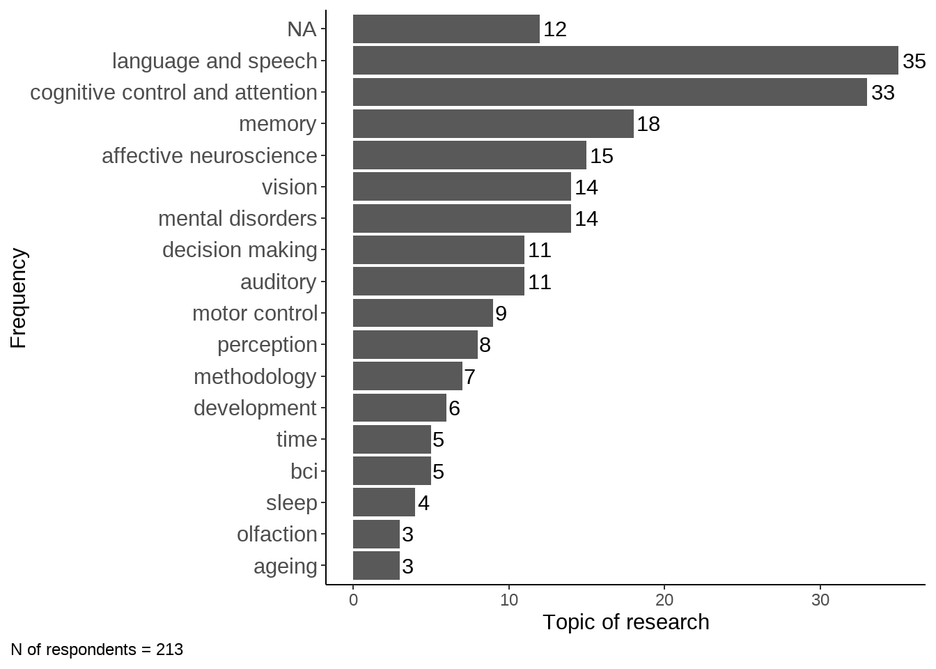

Experience

Years

Code

year <- data %>% dplyr::rename(years = !!names(.)[20]) %>% filter(.[[20]] < 50) %>% select(years)

years <- year %>% group_by(years) %>% 
  dplyr::summarise(n = n()) %>% 
  mutate(p = round(n / sum(n), 2))  %>% ggplot(data = ., aes(x=years, y = p)) +
  geom_col(position = "identity", col="grey") +  scale_x_continuous(breaks=seq(0, 30, 5)) +
  labs(x ="Years of experience with EEG, MEG, or iEEG analysis", y="") +
  theme_classic() + theme(legend.position="none", text = element_text(family = "Lato"),
                          axis.text = element_text(size = 10)) +
  theme(legend.position="none", plot.caption = element_text(hjust=0), 
        axis.text = element_text(size = 10)) + 
  geom_vline(xintercept = median(year$years),        # Add line for mean
             col = "brown1", lty='dashed',
             lwd = 1) +
  geom_text(aes(label = paste0("median = ", median(year$years)), col = "brown1",
                x = median(year$years)*2.2, family = "Lato",
                y  = 0.11)) + scale_y_continuous(labels = scales::percent)

years + labs(caption = sprintf("N of respondents - %d, median - %d", nrow(year), median(year$years)))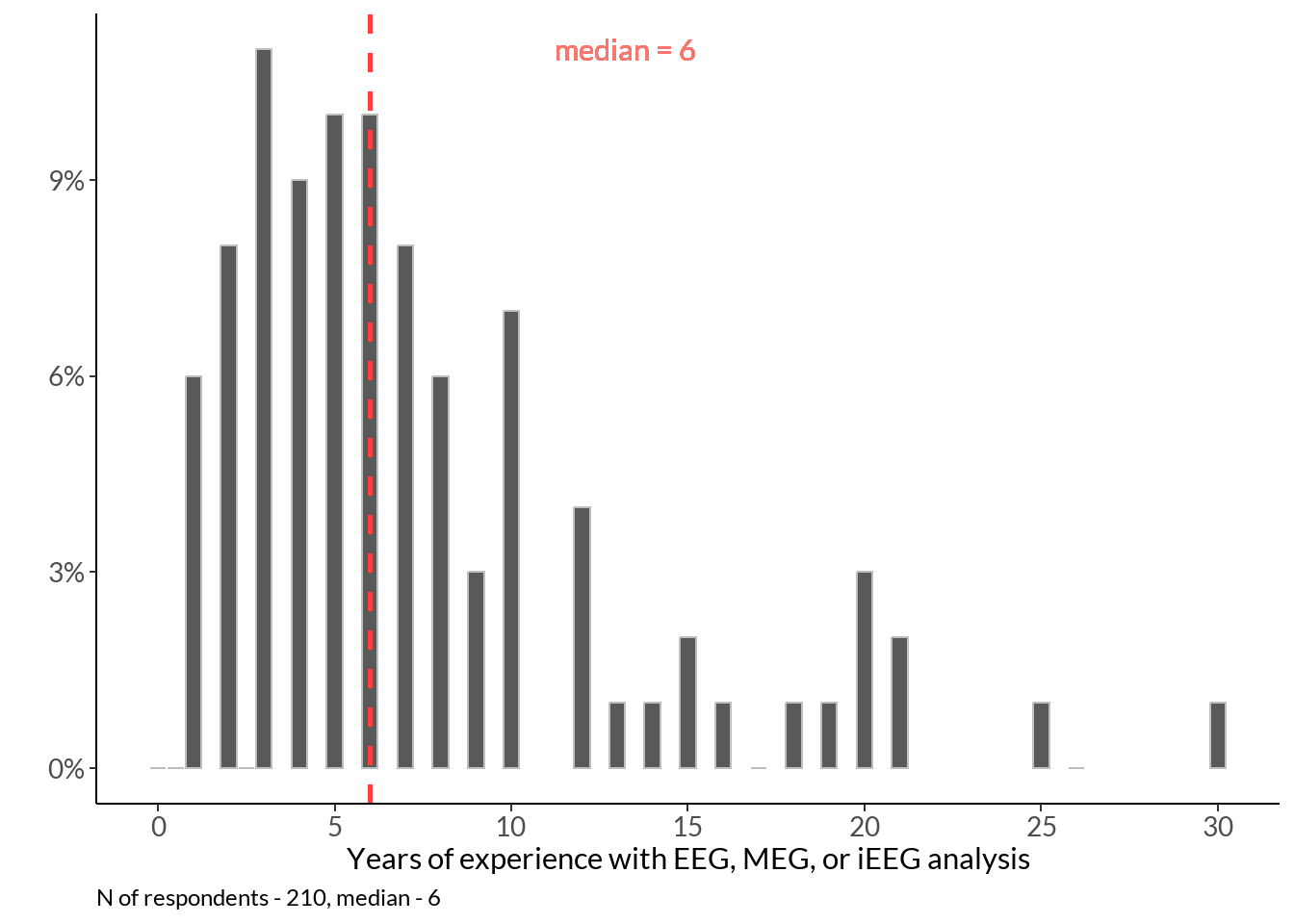  

Papers

Code

tmp_med <- data[19] %>% dplyr::rename(papers = !!names(.)[1]) %>% 
  filter(papers < 100) %>% summarise(median_paper = median(papers)) %>% as.numeric()

papers <- data[19] %>% dplyr::rename(papers = !!names(.)[1]) 

papers_fig <- papers %>% 
  filter(papers < 100) %>% group_by(papers) %>% 
  dplyr::summarise(n = n()) %>% 
  mutate(p = round(n / sum(n), 2)) %>% 

ggplot(., aes(x = papers, y = p)) +
  geom_col(position = "identity", bins = 45, col="grey") +
  labs(x ="The number of published papers/preprints with EEG, MEG or iEEG analysis", y = "") + theme_classic()  +
  theme(legend.position="none", plot.caption = element_text(hjust=0), text = element_text(family = "Lato"),
        axis.text = element_text(size = 10)) + 
  geom_vline(xintercept = tmp_med - 1,        # Add line for mean, -1 because starts from zero
             col = "brown1", lty='dashed',
             lwd = 1) +
  geom_text(aes(label = paste0("median = ", tmp_med), 
                x = tmp_med*7, col = "brown1", family = "Lato",
                y  = 0.15)) + scale_y_continuous(labels = scales::percent)
papers_fig +
  labs(caption = sprintf("N of respondents - %d, median - %s", nrow(papers), as.character(tmp_med)))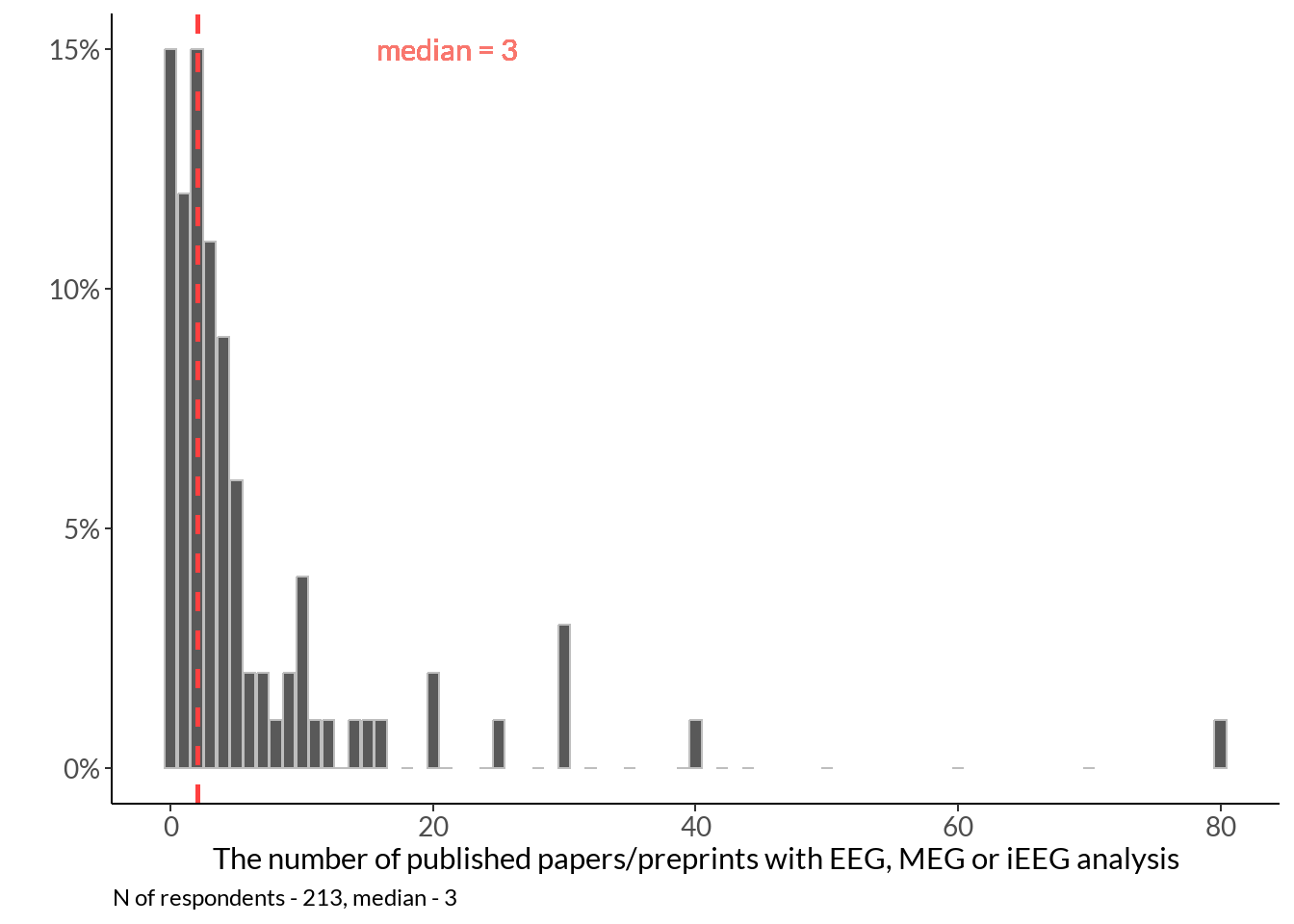

Self-assessed level

Code

colorsal <- c("#f9a65a", "#599ad3", "#8dc63f")
sal <- table(data[21]) %>% data.frame() %>% dplyr::rename(level = !!names(.)[1]) %>%
    mutate(percent_score = round(Freq / sum(Freq) * 100)) %>% 
    mutate(level = factor(level, levels = rev(c("Beginner", "Intermediate", "Expert"))))

sall <- sal %>% 
    ggplot(data = ., aes(y = level, x = percent_score)) +  
    geom_col(stat="identity",  width = 0.5) + labs(x = "Percent", y = "", title="Self-assessed level") +
    geom_text(aes(label = paste0(percent_score, "%")), hjust = -0.2)  + theme_classic() +
    theme(legend.position="none", axis.text.x = element_text(size = 12), text = element_text(family = "Lato"),
          plot.caption = element_text(hjust=0), axis.text = element_text(size = 10))
sall +
    labs(caption = sprintf("N of respondents - %d",  sum(sal$Freq))) + xlim(0, 50)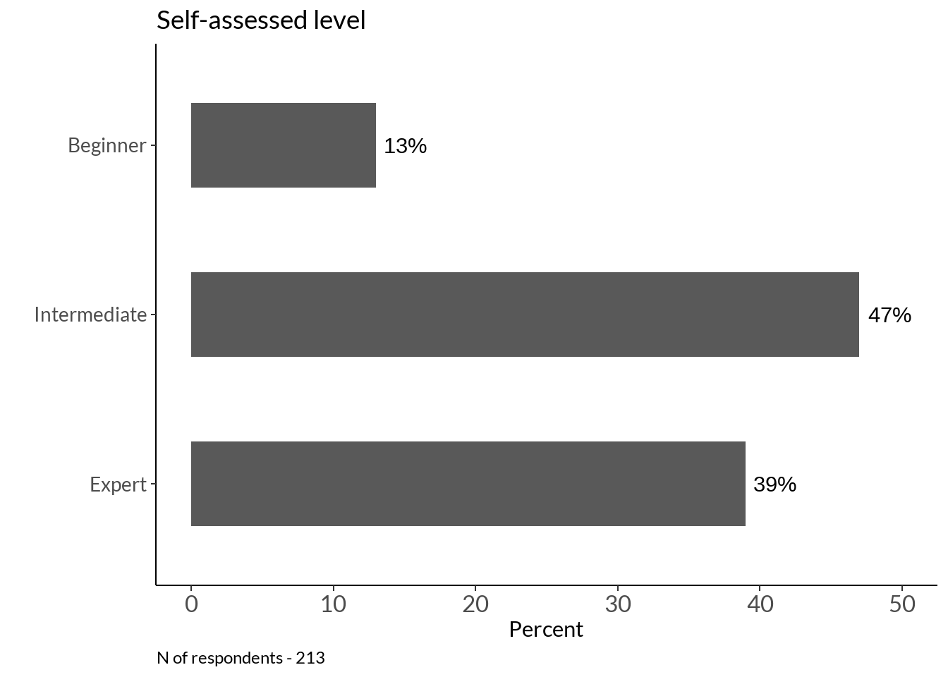

Code contribution

Code

cc <- table(data[22])  %>% data.frame()%>% dplyr::rename(level = !!names(.)[1]) %>%
    mutate(percent_score = round(Freq / sum(Freq) * 100)) %>% 
    ggplot(data = ., aes(y = reorder(level, Freq),  x = percent_score))  +
    geom_col(stat="identity", width = 0.5) + 
    geom_text(aes(label = paste0(percent_score, "%")), hjust = -0.2)  +
  theme_classic() +
  theme(legend.position="none", axis.text.x = element_text(size = 12), text = element_text(family = "Lato")) +
  labs(title = "Code contribution", x="Percent", y="")  +
    theme(legend.position="none", plot.caption = element_text(hjust=0), axis.text = element_text(size = 10)) + xlim(0, 64)
cc +
    labs(caption = sprintf("N of respondents - %d",  sum(sal$Freq)))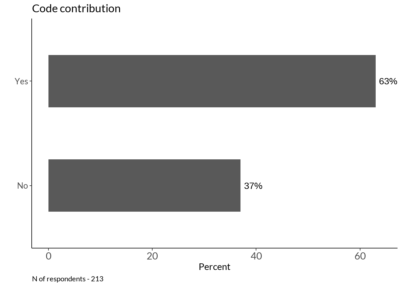 

Combined plots

Code

ggarrange(country_fig + geom_col(stat = "identity", width = 0.8, fill ="#6BAED6") + 
            theme(axis.text.y = element_text(size = 10), axis.text.x = element_blank()) + xlim(0, 100) + labs(x= "Percent of respondents"), 
          position + xlim(0, 100) + geom_col(stat = "identity", fill ="#6BAED6") + 
            theme(axis.text.y = element_text(size = 10), axis.text.x = element_blank()) + labs(x = "Percent of respondents"),   
          fieldplot + xlim(0, 100) + geom_col(stat = "identity", width = 0.7, fill ="#6BAED6") + 
            theme(axis.text.y = element_text(size = 10), axis.text.x = element_blank()) + labs(x = "Percent of respondents"), 
          methods  + geom_col(stat = "identity", width = 0.7, fill ="#6BAED6") +  
            scale_y_discrete(labels=c("OPMs", "iEEG", "MEG", "Scalp EEG")) + xlim(0, 100) +  
            theme(axis.text.y = element_text(size = 10), axis.text.x = element_blank()) + labs(x = "Percent of respondents"),
          labels = c("A", "B", "C", "D"),
          ncol = 2, nrow = 2, align = 'hv')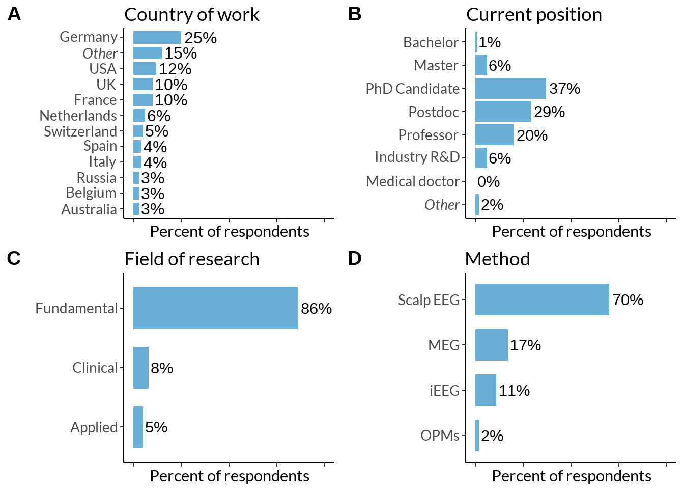  

Code

 #RColorBrewer::brewer.pal(8, "Reds")
#"#FFF5F0" "#FEE0D2" "#FCBBA1" "#FC9272" "#FB6A4A" "#EF3B2C" "#CB181D" "#99000D"

ggarrange(years +  geom_col(position = "identity", bins = 45, fill ="#6BAED6") + 
  geom_vline(xintercept = median(year$years),        # Add line for mean
             col = "#FC9272", lty='dashed',
             lwd = 1) + labs(title ="Years of experience", y= "Percent of\nrespondents", x="") ,
  
          papers_fig + geom_col(position = "identity", bins = 45, fill ="#6BAED6") + 
  geom_vline(xintercept = tmp_med - 1,        # Add line for mean
             col = "#FC9272", lty='dashed',
             lwd = 1) + labs(title ="Number of papers published", y= "Percent of\nrespondents", x=""), 
  
          cc +  geom_col(stat = "identity",  width = 0.5, fill ="#6BAED6") + xlim(0, 100) + theme(axis.text.y = element_text(size = 10), axis.text.x = element_blank()) +  
    labs(x ="Percent of respondents") , 
  
          sall + geom_col(stat = "identity",  width = 0.5, fill ="#6BAED6") + xlim(0, 100) + theme(axis.text.y = element_text(size = 10), axis.text.x = element_blank()) +  
    labs(x ="Percent of respondents"), 
          labels = c("A", "B", "C", "D"),
          ncol = 2, nrow = 2)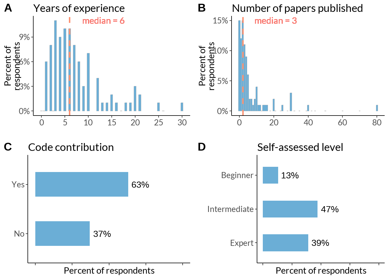 

Time of finishing survey in minutes

Code

median(as.numeric(as.matrix(data[121]))) / 60

[1] 13.86367